We will follow the toy model provided in Ref.22. The infinitesimal line element ds, whose coefficients determine the metric of the spacetime, in a Friedman–Lemaitre–Robertson–Walker universe is given by Refs.23,24,25,26,27,28,29:
$$\begin{aligned} ds^2=dt^2-a^2(t)dx^2, \end{aligned}$$
(1)
where a(t) is the scale factor, which only depends on time.
We can make a change of variables to conformal time, such that \(d\eta =\frac{dt}{a(t)}\), so the metric in these coordinates becomes:
$$\begin{aligned} ds^2=a^2(\eta )\left( d\eta ^2-dx^2\right) =C(\eta )\left( d\eta ^2-dx^2\right) , \end{aligned}$$
(2)
where \(C(\eta )=a^2(\eta )\), which is obtained by substituting time t for conformal time \(\eta\) through solving the following integral:
$$\begin{aligned} \eta =\int \frac{dt}{a(t)}. \end{aligned}$$
(3)
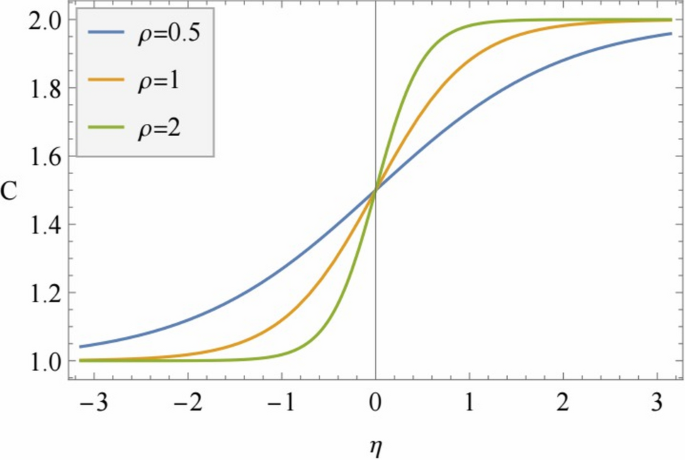
We work in a universe that evolves from a stationary state where \(C(-\infty )=A-B\) to a new stationary state where \(C(\infty )=A+B\) through \(C(\eta )=A+B\tanh (\rho \eta )\), where \(\rho >0\) is a constant that codifies the transition velocity (see Fig. 1). The universe expands if \(B>0\), contracting otherwise. The value of \(C(\eta )\) must always be positive, so \(A>|B|\).
Scale factor as a function of time for a universe that expands with a speed \(\rho =0.5\) (blue), \(\rho =1\) (orange), and \(\rho =2\) (green), with \(A=1.5\) and \(B=0.5\).
On this gravitational background, we place a free scalar field with mass m, that is, it evolves over time through the Klein–Gordon equation30,31:
$$\begin{aligned} \frac{\partial ^2\phi }{\partial \eta ^2}-\frac{\partial ^2\phi }{\partial x^2}+C(\eta )m^2\phi =0. \end{aligned}$$
(4)
This partial differential equation can be solved by separation of variables, with a solution for each mode of the form:
$$\begin{aligned} \phi _k(\eta , x)=\frac{1}{\sqrt{2\pi }}e^{ikx}\chi _k(\eta ), \end{aligned}$$
(5)
with \(\chi _k(\eta )\) satisfying:
$$\begin{aligned} \frac{d^2\chi _k}{d\eta ^2}+\left( k^2+C(\eta )m^2\right) \chi _k=0, \end{aligned}$$
(6)
whose solution is given by hypergeometric functions.
We are particularly interested in the behavior of the field in the limits \(\eta \rightarrow \pm \infty\), which is given by:
$$\begin{aligned} & \phi _k(\eta \rightarrow -\infty , x)\rightarrow \frac{1}{\sqrt{4\pi \omega _{in}}}e^{i\left( kx-\omega _{in}\eta \right) }, \end{aligned}$$
(7)
$$\begin{aligned} & \phi _k(\eta \rightarrow \infty , x)\rightarrow \frac{1}{\sqrt{4\pi \omega _{out}}}e^{i\left( kx-\omega _{out}\eta \right) }, \end{aligned}$$
(8)
where \(\omega _{in}=\sqrt{k^2+m^2(A-B)}\) and \(\omega _{out}=\sqrt{k^2+m^2(A+B)}\). These two limits are of special interest because \(\omega _{out}\), the frequency of the free field after the expansion, is the frequency that will appear in the Hamiltonian governing the time evolution of the field after the universe expands. Additionally, together with \(\omega _{in}\), these are the frequencies that are needed to relate the vibrational modes of the field before and after the expansion, which is crucial for computing the number of particles created by the expansion of the universe.
Clearly, the vibration modes of the field are not the same before and after a short period of inflation. Initially, the field is stationary in the vacuum state \({|{0, in}\rangle }\). After the inflationary evolution, however, this state is not going to be an eigenstate of the time evolution anymore, so we could detect a number of particles different from zero and study their evolution over time.
We have chosen this model because the vibration modes of the field before inflation can be easily related to those after inflation, in the sense that the vibrations with momentum k mix only with their opposite \(-k\), but not with other configurations with different |k|. The Bogoliubov transformations that relate the vibration modes \(\phi ^{in}\) and \(\phi ^{out}\) are given by:
$$\begin{aligned} \phi _k^{in} = \alpha _k \phi _k^{out} + \beta _k \phi _{-k}^{out*}, \end{aligned}$$
(9)
where the coefficients \(\alpha\) and \(\beta\) are complex functions of \(\omega _{in}\), \(\omega _{out}\) and \(\rho\)22:
$$\begin{aligned} \alpha _k = \sqrt{\frac{\omega _{out}}{\omega _{in}}} \frac{\Gamma \left( 1-i\frac{\omega _{in}}{\rho }\right) \Gamma \left( -i\frac{\omega _{out}}{\rho }\right) }{\Gamma \left( -i\frac{\omega _+}{\rho }\right) \Gamma \left( 1-i\frac{\omega _+}{\rho }\right) }, \quad \quad \quad \quad \beta _k = \sqrt{\frac{\omega _{out}}{\omega _{in}}} \frac{\Gamma \left( 1-i\frac{\omega _{in}}{\rho }\right) \Gamma \left( i\frac{\omega _{out}}{\rho }\right) }{\Gamma \left( i\frac{\omega _-}{\rho }\right) \Gamma \left( 1+i\frac{\omega _-}{\rho }\right) }, \end{aligned}$$
(10)
with \(\omega _\pm =\frac{1}{2}\left( \omega _{out}\pm \omega _{in}\right)\).
The reason why we are using this toy model to simulate the cosmological particle production is because its simplicity allows us to write an analytical expression for the Bogoliubov coefficients, which relate the vibrational modes of the field, and its respective quantized observables, before and after the expansion. For other models whose relationship between modes is not known, it is not possible to perform such simulations. Furthermore, in more general models of QFTCS, the number of particles is not well-defined, depending on the observer measuring it. A classical example of this is black hole thermal radiation, which is zero for a near-horizon freely falling observer, but non-zero for a stationary one. In contrast, our model allows us choose an observer who initially detects the vacuum and study the particle creation from its perspective.
When quantizing the field, we use the annihilation and creation operators \(a_+\) and \(a_+^\dagger\) for the in modes of positive k, and \(a_-\) and \(a_-^\dagger\) for the in modes of negative k. These creation and annihilation operators are related to the annihilation and creation operators of the out modes, which we call \(b_+\), \(b_+^\dagger\), \(b_-\) and \(b_-^\dagger\), using the same Bogoliubov coefficients32,33:
$$\begin{aligned} & b_+ = \alpha a_+ + \beta ^* a_-^\dagger \quad \quad \quad \quad b_+^\dagger = \alpha ^* a_+^\dagger + \beta a_-, \end{aligned}$$
(11)
$$\begin{aligned} & b_- = \alpha a_- + \beta ^* a_+^\dagger \quad \quad \quad \quad b_-^\dagger = \alpha ^* a_-^\dagger + \beta a_+. \end{aligned}$$
(12)
Now, the generator of the time evolution of these two positive and negative modes is the Hamiltonian:
$$\begin{aligned} \begin{aligned} \hat{\mathcal {H}}&= \hbar \omega _{out} \left( b_+^\dagger b_+ + b_-^\dagger b_- \right) \\&= \hbar \omega _{out} \left( \alpha \alpha ^* \left( a_+^\dagger a_+ + a_-^\dagger a_- \right) + \beta \beta ^* \left( a_+ a_+^\dagger + a_- a_-^\dagger \right) + 2 \alpha ^* \beta a_+^\dagger a_-^\dagger + 2 \alpha \beta ^* a_+ a_- \right) . \end{aligned} \end{aligned}$$
(13)
In the interaction picture, an initial vacuum state will evolve under the interaction hamiltonian:
$$\begin{aligned} \mathcal {H}_{int} = 2 \hbar \omega _{out} \alpha \beta ^* a_+ a_- + h.c. \end{aligned}$$
(14)
Thus the time evolution operator in this picture is:
$$\begin{aligned} U = e^{i \omega _{out} t \left( 2 \alpha \beta ^* a_+ a_- + h.c. \right) }. \end{aligned}$$
(15)
We are interested in the number of particles—as defined before the expansion by the in operators- created after the expansion as a function of the expansion rate \(\rho\).
This type of particle creation process due to a non-flat metric can be interpreted as if the field were in thermodynamic equilibrium with a thermal source34,35. Therefore, the state predicted by quantum field theory for the time evolution operator 15 applied to an initial vacuum is a state well-known in quantum optics—two-mode squeezed state36 where \(2 \alpha \beta ^* \omega _{out} t\) is the squeezing parameter. When the trace over one mode is taken over a two-mode squeezed state, a single-mode thermal state with squeezing-dependent temperature is obtained37, giving rise to:
$$\begin{aligned} \rho = \frac{1}{\cosh ^2 \left( 2 \left| \alpha \right| \left| \beta \right| \omega _{out} t \right) } \sum _{n=0}^\infty \tanh ^{2n} \left( 2 \left| \alpha \right| \left| \beta \right| \omega _{out} t \right) {|{n}\rangle } {\langle {n}|}. \end{aligned}$$
(16)
Therefore, the expected number of particles created can be calculated as:
$$\begin{aligned} \left\langle {n}\right\rangle = \sinh ^2\left( 2\left| \alpha \right| \left| \beta \right| \omega _{out}t\right) . \end{aligned}$$
(17)
As we will see below, we will restrict ourselves to only one created particle per mode. The state restricted to one excitation can be obtained by taking the first two terms of the sum in (16) and renormalizing, giving rise to:
$$\begin{aligned} \left\langle {n}\right\rangle = \frac{\tanh ^2 \left( 2 \left| \alpha \right| \left| \beta \right| \omega _{out} t \right) }{1 + \tanh ^2 \left( 2 \left| \alpha \right| \left| \beta \right| \omega _{out} t \right) }. \end{aligned}$$
(18)