Morphology of ejecta features from the impact on asteroid Dimorphos

Methodology overview

A schematic overview of the methodology is reported in Supplementary Fig. 3. More details on data and functional blocks reported in the Figure, as well as the full simulation/processing pipeline are provided in the next paragraphs. Numerical tools used to propagate the dynamics of the ejecta and for the analysis of images are developed internally at Politecnico di Milano.

The dynamics of ejecta particles are simulated under the gravitational influence of Didymos, Dimorphos and the Sun, and the SRPs. More details are found in the Dynamical simulations subsection. Overall, 30 simulation sets were run, each propagating trajectories of 5 million ejecta particles, using a high-fidelity model of their dynamics and ephemerides of the Sun and asteroids⁶. The range of particle radii was selected after some preliminary simulations, to ensure it contains ejecta involved in the formation of the features reported below. This was needed to avoid severe computational burdens, while still considering a representative subset of ejecta that can be compared with observations. Due to the impossibility to simulate all particles involved, we use an image multiplication procedure to compensate for this issue⁵¹. The multiplicative compensation procedure, as detailed in its dedicated subsection, weights each simulated ejecta particle as a cluster of particles according to the total mass and the dSFD coefficient. The multiplicative compensation procedure output is a series of image multipliers which modifies the radiative flux of each HST pixel according to the particle size and the ejecta total mass. Indeed, we consider these two parameters as the ejecta characteristics to be determined with a parametric analysis reported hereafter. More details about the multiplicative compensation procedure are reported below.

From these inputs, we performed a preliminary investigation to identify the most suitable set of simulations in terms of ejecta dynamical parameters (i.e., the ejecta velocity-size distribution). This investigation has been performed by rendering images with coarse values of ejecta total mass (i.e., 10⁶ kg and 10⁷ kg) and one dSFD coefficient (i.e., −2.7) and by comparing visually the cone-related and tail-related features between real and synthetic images. The synthetic rendered images are generated by emulating the observational geometry of the HST and by assuming the photometrical ejecta characteristics from the literature^51,52,53,54. More details about the rendering procedure are reported below. We performed a preliminary selection of simulations focusing on the timing of features and their appearance by visual inspection. We identified that the tail- and the cone-related features are associated with different velocity ranges. Examples of discarded simulations are reported in Fig. 5. We use the selected dynamical parameters to simulate a dataset of synthetic images by varying over a finer grid of total ejecta mass and dSFD coefficients, generating a large dataset of synthetic images to be compared against HST real images. We perform this comparison by computing the radiometric flux error. The radiometric flux error is defined as the sum of the error between the flux in each pixel of the simulated image and the HST image over all the considered pixels. As we are interested in only some specific region of the HST images, we perform this sum only on some areas defined by a coarse label identifying three main regions in the HST image: the noise mask, the cone-related mask, and the tail-related mask. More details about each mask are provided in the following paragraphs. The cone-related and tail-related masks are used to compute the radiometric flux error for the associated features in a neighbor of the HST feature location. The noise mask is used to estimate the mean level of image noise. This provides a threshold to the radiometric flux, and values below this threshold do not contribute to the photometric error. We perform this step as the rendered images are noiseless and we need to avoid overfitting of the rendered data with HST image noise. This procedure is used to compute numerical values reported Fig. 6, which in turn is used to select the total ejecta mass and dSFD coefficient for both the cone-related feature and the tail-related feature.

Finally, we render a final image merging the cone-related and tail-related velocity distributions considering its respective the total ejecta mass and its respective dSFD coefficient. These rendered images are the ones shown in Figs. 2 and 4. We use these final images to extract the best-fit simulation data reported in Table 1 by using a set of high-fidelity masks. The high-fidelity masks are computed by labeling HST images to identify detailed areas where each feature is located. More details about these masks and the labeling are reported below.

Label generation

The main goal of this step is to generate two sets of labels: the coarse masks and the Hi-Fi masks. In the text we will refer to image labels or image masks as synonyms. These two image masks are used for different applications. The formers are exploited to compute the radiometric flux error, while the latter are used to compute the ejecta morphological characteristics reported in Table 1.

To gather the image labels, the set of 16 short-exposure images acquired by HST after the impact is used to extract the masks. The features are identified manually on the images using the “Image Labeler” tool by Matlab. Once identified, the annotated labels act as a mask, that can be applied logically to the projected simulation results to quantify physical properties associated with them.

For the coarse labeling step, three main masks are identified in the HST images:

1. 1.

   The noise mask is the image region where no information about the cone-related and tail-related features is present. Therefore, this area is used to gather the mean image error to compute the radiometric flux error

2. 2.

   The tail-related mask which contains the information linked with the tail

3. 3.

   The cone-related mask which contains the information linked with the ejecta spiraling behavior

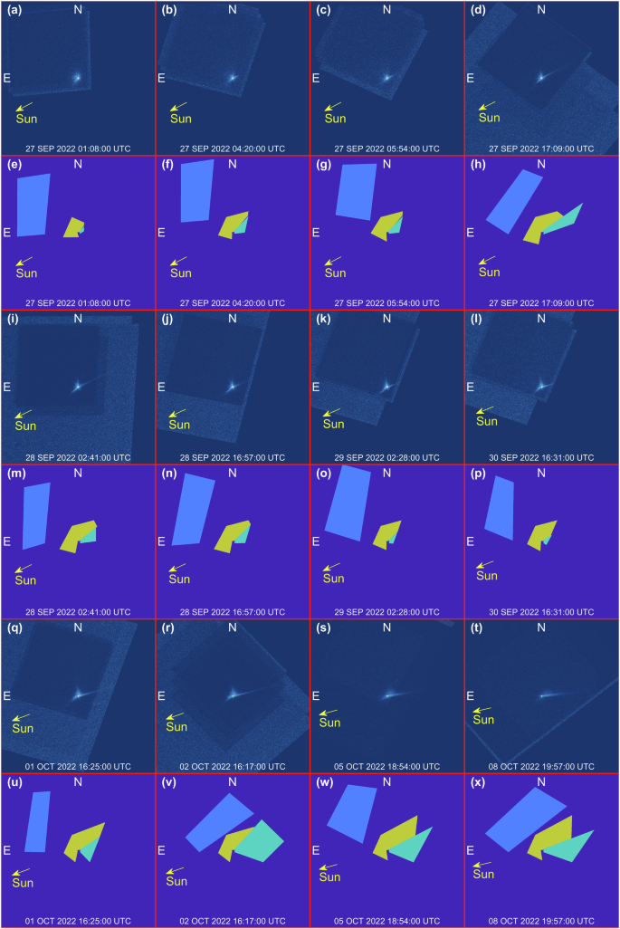
Examples of the coarse labels are shown in Fig. 8 along with the real HST image. Note that the cone-related and the tail-related labels include not only the area where the associated feature are present, but also a region of the image where this feature is not present. This is done to penalize simulations where the ejecta in the simulated images are more spread around with respect to the real HST images. Indeed, when this occurs, the radiometric flux error increases avoiding converging to a wrong solution.

For the high-fidelity labeling step, five main masks are labeled which are associated with five main features:

1. 1.

   The central blob of pixels which is the brightest area in the image. This image region is associated with the Didymos system

2. 2.

   The spiral North front which is the portion of the cone-related features ejected from Dimorphos in the direction of Didymos (i.e., the North as projected in the HST image)

3. 3.

   The spiral South front which is the portion of the cone-related features ejected from Dimorphos in the direction opposite of Didymos (i.e., the South as projected in the HST image)

4. 4.

   The tail which is composed of both the primary and secondary tail (when present)

5. 5.

   The background which is defined as the image region complementary to all other labels.

Figure 9 shows examples of the high-fidelity labels along with the prelabeled HST images. These labels are used to postprocess the final rendered image to compute morphological characteristics as the ones reported in Table 1.

Dynamical simulations

We assume that Didymos and Dimorphos do not feel the gravitational effects of the ejecta, although a significant quantity of bound ejecta could subtly affect the binary orbit period³⁸, as mentioned above. However, this is not relevant for the dynamical evolution of DART ejecta features. To perform dynamical simulations, we use a quasi-inertial reference frame centered at the binary system barycenter. Axes are inertially fixed, with X and Y lying on the ecliptic plane at epoch J2000, and Z completing the orthogonal triad. The use of prefix quasi highlights how the system should be considered inertial for characteristic times shorter than the Didymos heliocentric revolution period³⁰. The dynamics of particles are driven by the central gravity field of Didymos and Dimorphos, the third-body effect of the Sun, and the SRP. Celestial bodies positions are resolved precisely, as provided by high-order integration in NASA’s DART mission kernels⁶. In our simulations, particles are assumed to be homogeneous and of spherical shape. Their mutual gravitational interactions are neglected. The dynamical propagator was developed at Politecnico di Milano and is coded in MatLab.

The equations of motion for a point mass (i.e., a particle) in the proximity of Didymos system read⁵⁵

Where \({\mu }_{D1}=3.490\times {10}^{-8}\,{{{\rm{k}}}}{{{{\rm{m}}}}}^{3}{{{{\rm{s}}}}}^{-2}\,\), \({\mu }_{D2}=3.246\times {10}^{-10}\,{{{\rm{k}}}}{{{{\rm{m}}}}}^{3}{{{{\rm{s}}}}}^{-2}\), and \({\mu }_{S}=1.327\times {10}^{11}\,{{{\rm{k}}}}{{{{\rm{m}}}}}^{3}{{{{\rm{s}}}}}^{-2}\) (refs. ^5,38) are the gravitational parameters of Didymos, Dimorphos, and the Sun, respectively; \({{{\bf{r}}}}\), \({{{{\bf{r}}}}}_{D1}\), \({{{{\bf{r}}}}}_{D2}\), and \({{{{\bf{r}}}}}_{S}\) are the position vectors of the particle, Didymos, Dimorphos, and the Sun with respect to the binary system barycenter, respectively. Lastly, the ballistic coefficient \(\beta={P}_{0}{D}_{{Au}}^{2}{C}_{r}^{*}/\left(c{\mu }_{S}\right)\) where⁵⁶ \({P}_{0}=1367\,{{{\rm{W}}}}{{{{\rm{m}}}}}^{-2}\) is the solar flux at 1 AU; \({D}_{{AU}}=1.495\times {10}^{8}{{{\rm{km}}}}\) is the Sun–Earth distance; \(c=2.998\times {10}^{8}\,{{{\rm{m}}}}{{{{\rm{s}}}}}^{-1}\) is the speed of light in vacuum; \({C}_{r}^{*}={C}_{r}A/m={3C}_{r}/\left(4R\rho \right)\) with \({C}_{r}\) the reflectivity coefficient, \(A\) the equivalent surface area, \(m\) the mass, R the radius, and \(\rho\) the density of the particle, set to 3.5 g/cm³ to match the grain density of L and LL chondrites⁵⁷, which are the best meteoric analogs for Didymos^58,59. The equations of motion are integrated with a multistep, variable-step, variable-order, Adams–Bashforth–Moulton, predictor-corrector solver of orders 1st–13th⁶⁰. The dynamics are propagated with relative and absolute tolerances both set to \({10}^{-9}\).

We propagate several sets of initial conditions. Each set contains \({N}_{p}={10}^{6}\) particles for each of the \({N}_{R}=5\) size distribution ranges \(\left[{R}_{i},\,{R}_{i+1}\right]\) with \({R}_{i}={10}^{-6+i}\) meter for \(i=0,\ldots,\,4\). A certain fraction of the particles are assumed to be isotropic ejecta, while the remaining fraction are arranged in a cone. Several isotropic/cone partition levels have been tested. However, isotropic particles were finally removed as their contribution was not in agreement with HST observations.

Each particle initial condition is constructed as follows:

1. i.

   sampling the particle radius \(R\) from \({{{\mathscr{U}}}}\left({R}_{i},\,{R}_{i+1}\right)\), where \({{{\mathscr{U}}}}\left(a,{b}\right)\) is the uniform distribution bounded in \(\left[a,{b}\right]\);

2. ii.

   assigning the DART spacecraft impact location as the initial position \({{{{\boldsymbol{r}}}}}_{0}\);

3. iii.

   computing the magnitude of the initial velocity \({v}_{0}=||{{{{\bf{v}}}}}_{0}||\) at the impact epoch \({t}_{0}\) for a particle belonging to:

   1. a.

      the isotropic contribution as a random velocity sampled from \({{{\mathscr{U}}}}\left({v}_{{esc}},\,2{v}_{{esc}}\right)\), where \({v}_{{esc}}\) is the Didymos escape speed from the impact point;

   2. b.

      the cone as the sum of the Didymos escape speed from the impact point \({v}_{{esc}}\) and a term dependent on the particle radius \({v}_{{radius}}\):

   $$v={v}_{{esc}}+\varrho {v}_{{radius}}$$

   (2)

   where \(\varrho\) is a multiplicative coefficient sampled from the uniform distribution \({{{\mathscr{U}}}}\left(0,\,1\right)\) and \({v}_{{radius}}\) is sampled from the velocity-size distribution (VSD) given by:

   $${\pi }_{v}\left(r\right)=\kappa {r}^{-\gamma }$$

   (3)

   where \(\kappa\) and \(\gamma\) are the coefficient and exponent, respectively, of velocity-size distribution, and \(r\) is the particle radius in meters.

4. iv.

   calculating the initial velocity direction \({\hat{{{{\bf{v}}}}}}_{0}=\,{{{{\bf{v}}}}}_{0}/{v}_{0}\) for particles belonging to:

   1. a.

      the isotropic contribution as \({\hat{{{{\bf{v}}}}}}_{0}={\left[\sqrt{1-{z}^{2}}\cos \phi,\sqrt{1-{z}^{2}} \sin \phi,{z}\right]}^{\top }\) with \(z\) and \(\phi\) sampled from distributions \({{{\mathscr{U}}}}\left(0,\,1\right)\) and \({{{\mathscr{U}}}}\left(0,\,2\pi \right)\), respectively, such that it belongs to the hemisphere facing the ejecta release direction and having the pole aligned with the DART spacecraft velocity at the impact epoch \({t}_{0}\);

   2. b.

      the cone as \({\hat{{{{\bf{v}}}}}}_{0}={[\sqrt{1-{z}^{2}}\cos \phi,\sqrt{1-{z}^{2}}\sin \phi,{z}]}^{\top }\) with \(z\) and \(\phi\) sampled from distributions \({{{\mathscr{U}}}}\left(\cos {\theta }_{1},\,\cos {\theta }_{2}\right)\) and \({{{\mathscr{U}}}}\left(0,\,2\pi \right)\), respectively, such that it is bounded between two coaxial cones with half-angles \({\theta }_{1}=60\) deg and \({\theta }_{2}=70\) deg, and axis aligned with the DART spacecraft velocity at the impact epoch \({t}_{0}\);

5. v.

   converting the initial position \({{{{\bf{r}}}}}_{0}\) and velocity \({{{{\bf{v}}}}}_{0}\) from the frame centered at Dimorphos to the frame centered at the binary system barycenter.

Supplementary Table 1 summarizes the velocity scaling power law \(\left(\kappa,\gamma \right)\) pairs selected to sample the random contribution \({v}_{{rand}}\) of the particle initial velocity, while a plot of the VSD is reported in Supplementary Fig. 1. The maximum velocity (corresponding to the minimum radius \(R={10}^{-6}\) m) of the distribution is reported as well.

Multiplicative compensation procedure

As previously mentioned, it is not possible to simulate the number of ejecta particles involved in the simulation, given their large number. We exploited and extended a preexisting methodology developed to simulate a smaller number of particles⁵¹. This implies the calculation of some multiplicative compensation factors that are used to weight each simulated ejecta particle as a pack of particles according to the total mass and the dSFD coefficient. The main steps of the used methodology are expounded hereunder.

We define \({\pi }_{N}(r)\) as the ejecta dSFD between a minimum radius \({r}_{m}\) and a maximum radius \({r}_{M}\) and normalized in such a way that its integral is equal to 1. Its expression is:

where \(r\) is the particle radius and \(a\) is the dSFD coefficient. Note that the SFD is the integral of the dSFD.

Let \(M\) be the ejecta total mass and \(N\) the total number of particles. The total mass can be computed as:

where \(V\left(r\right)\) is the particle volume as a function of \(r\) and \(\rho\) is the particle density assumed constant. By assuming the total ejecta mass and the dSFD coefficient, it is possible to derive the total number of particles between \({r}_{m}\) and \({r}_{M}\):

Note that the SFD coefficient \(a{\prime}\) is related with the dSFD coefficient \(a\) by \({a}^{{\prime} }=a-1\). At this stage it is necessary to compute the multiplicative compensation factors which depends on the particle radius. Indeed, particles must be weighted according to the selected dSFD as a single particle represent a pack of particle which are distributed according to \({\pi }_{N}(r)\). To ease the calculations, we divide the interval \([{r}_{m},\,{r}_{M}]\) in subintervals. Let \({r}_{{l}_{i}}\) and \({r}_{{u}_{i}}\) be the lower and upper bound of the ith bin. The fraction of particles within the i th bin is labeled \({n}_{i}\) and it is computed as:

Let \({N}_{{{{{\rm{sim}}}}}_{i}}\) be the number of effective particles simulated within the ith bin. It is straightforward to compute the multiplicative compensation factor \({k}_{i}\) each ejecta particle has so to match the desired fraction of particle in that bin with a given total ejecta mass and dSFD coefficient:

Note that this multiplicative compensation factor is constant within the same bin, implying that particles with different radii are weighted in the same manner. Moreover, we used the mean particle radius within the considered bin to render ejecta particles avoid small faint particle which are weighted as larger bright particles. To average the behavior of the particle within the same bin, we decided to add a second computational step to infer the multiplicative compensation factor \({k}_{i}\). We use the fraction of particles within the ith bin \({n}_{i}\) to define a piecewise constant function \({\bar{\pi }}_{N}(r)\) representing the dSFD defined between \({r}_{m}\) and \({r}_{M}\) and normalized in such a way that its integral its equal to 1. This function is constant within the bin defined by \({r}_{{l}_{i}}\) and \({r}_{{u}_{i}}\) and it contains \({n}_{i}\) percentage of the total particle. It can be expressed as follows:

where \({\mathbb{I}}({{\bullet }})\) is the indicator function, defined as 1 in the input interval; 0 otherwise.

The total ejecta mass is:

where \(\bar{N}\) is the total number of particles associated with the distribution \({\bar{\pi }}_{N}(r)\). Therefore, \(\bar{N}\) is computed as:

The multiplicative compensation factor \({\bar{k}}_{i}\) associated with the distribution \({\bar{\pi }}_{N}(r)\) are computed as:

These are the multiplicative compensation factors we use to weight each particle in the simulations according to the bin where it belongs to.

Synthetic image generation

To perform synthetic image generation, we simulate the HST with a pinhole camera model⁶¹ with focal length of 57.6 m, an iFoV (instantaneous Field of View) of 0.194 μrad in both directions and resolution of 2001 pixels in both directions⁵¹. The first step we apply is to compute which particles fall within the HST field of view to reduce the calculation in projecting them in the image plane. Then we project all the filtered particle on the image plane to identify which pixel is associated with the considered particle. Per each particle we compute the ejecta particle visual magnitude at HST observational geometry \({m}_{{{{\rm{particle}}}}}\):

where \({m}_{1,0}\) is the particle magnitude at 1 AU from Sun and observer with zero phase angle, \({d}_{P,{C}}\) is the distance between the particle and the camera in AU, \({d}_{P,{S}}\) is the distance between the particle and the Sun in AU, and \(G(\alpha )\) is a phase function correcting for phase angle \(\alpha\). We use the following phase function⁵²:

where \(\alpha\) is expressed in degree. Moreover, we compute the magnitude of the particle at 1 AU with zero phase angle as^51,53:

where \({r}_{{{{\rm{particle}}}}}\) is the particle radius expressed in mm and \(a\) is the particle albedo assumed 0.15. Note that we divide the considered range of particle radius in several bins to ease the computation of the multiplicative compensation factor \({\bar{k}}_{i}\). As all particles are weighted equally in the same bin, we use the mean particle radius of the bin to avoid giving more importance to larger particle in the same bin.

We compute the radiometric flux \(E\) by using Vega reference parameters:

where \({m}_{{{{\rm{Vega}}}}}\,\)= 0.03 is the Vega magnitude, \({E}_{{{{\rm{Vega}}}}}\) = 3.631 × 10⁻⁸ W/(m² nm) is Vega reference irradiance in the visible. At this stage we sum all radiometric flux contributions in the same pixel coming from the particles in the same bin and we multiply these values for the multiplicative compensation factor \({\bar{k}}_{i}\). Moreover, we sum up all the contributions coming from different bins to obtain the image for all the simulated ejecta. Finally, to consider the HST WFC3 F350LP filter and obtain images in the same units of HST data, we perform the following calculations:

where \(I\) is the rendered image, \({I}_{{{{\rm{final}}}}}\) is the final image coherent with HST data, and \({E}_{{{{\rm{Filter}}}}}\) = 2.7554 × 10⁻⁸ W/(m² nm) is the F350LP filter zero point.