Hardware and software
The following list summarizes the key hard- and software components used for acquiring the results.
-
Laser: neoLASE neoMOS, 50 kHz–20 MHz, M2 = 1.15, 10 ps
-
Laser power infrared: P = 41.3 W@1MHz, P = 28.1W@100kHz, green: P = 17W@1MHz, P = 11W@100kHz
-
Receive telescope 1: Contraves, Cassegrain, d = 0.5 m, for monostatic setup
-
Receive telescope 2: ASA, Ritchey-Chretien, d = 0.8 m, for bistatic setup
-
Transmit telescope: Contraves, d1 = 0.07 m, monostatic and bistatic setup
-
Detector: Micro Photon Devices Photon Counter d = 100 μm, Grade A 500 cps
-
Filter 1: Thorlabs, TL FLH532-1, FWHM = 1.0 nm
-
Filter 2: Alluxa, optical density 6, FWHM = 0.19 nm
-
Range gate generator: Altera Cyclone V GX FPGA
-
Event timer 1: Eventech A033-ET/USB, monostatic setup
-
Event timer 2: Swabian Instruments Time Tagger Ultra, bistatic setup
-
Timing: Brandywine NFS220 plus, 10 MHz/1 pps clock
-
Post-processing software: Python, self-developed
-
SLR ranging software: C++, self-developed
Noise level comparison: 100 kHz vs. 1 MHz
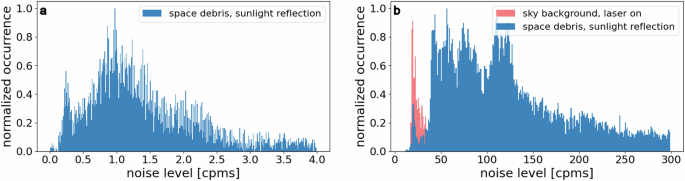
For all successful passes at 100 kHz monostatic and 1 MHz bistatic, the noise level was analyzed. By selecting only successful debris passes (passes with clear returns) it can be ensured that the sunlight reflection of the target is contributing to the noise. The overall number of photon counts per meter and second (cpms), including noise and signal, is evaluated and the occurrence calculated and displayed by means of a histogram plot (Fig. 6, blue). For 100 kHz (monostatic) the noise level peaks at approximately 1 cpms. Depending on the brightness of the target the noise level increases up to 2.5 cpms. At 1 MHz (bistatic) the average noise level is larger, with multiple distinguishable peaks between ~50 and 120 cpms. As the overall number and variety of targets was larger (17 successful passes for 1 MHz), the individual peaks are expected to belong to different object sizes. At ~20 cpms an additional small peak is visible, connected to low noise conditions. To investigate the reason for this behavior, at 1 MHz for a full pass just background sky noise was recorded. A LEO space debris target was tracked with a large offset to ensure that the object was well outside of the field of view of the receiving path. During the whole pass, the laser was on and the laser energy was periodically varied to see if backscatter has any effect on the noise. The recorded noise data showed no periodic variation, which proves that the receiving telescope is outside the backscatter region. Adding the sky noise measurement data to the histogram (Fig. 6b, red) shows that the noise level due to the sky is exactly at the same location as the first peak in the dataset based on analyzing illuminated debris objects. We conclude that this peak corresponds to observation conditions where the target is invisible or outside the field of visible. This marks the minimum noise condition for the current bistatic observation settings.
Histogram distribution of the background noise level of all successful space debris laser ranging passes at a 100 kHz monostatic and b 1 MHz bistatic. The noise counts per meter and second (cpms) are plotted with respect to the normalized occurrence. The noise connected to illuminated space debris (blue) for 1 MHz is by a factor of 50-100 larger as compared with 100 kHz. A noise measurement of the sky background (red) reveals the minimal noise level which is present in both distributions. During the sky measurement the laser power was varied periodically without any influence on the noise level, verifying that the receiving station does not detect laser backscatter in bistatic configuration.
Compared to 100 kHz in monostatic mode (50 kHz effectively due to burst mode), the noise level at 1 MHz is by a factor of ~50–100 larger. A factor of 20 can be explained by the difference in repetition rate. The rest is expected to come from the larger aperture of the bistatic receiving telescope (80 cm vs. 50 cm).
Signal to noise at different repetition rates
The bistatic results of Jason-2 reveal that MHz repetition rate plays out its true strength when operating in the single photon regime at large return rates. Ideally each laser pulse should just carry enough energy to deliver single photons to the detector. Once operating in the multi-photon level, excessive pulse energy will reduce the overall returns per second, which is limited by the power of the laser. This intuitive explanation holds if the signal is much bigger than the underlying noise level. As seen before (Figs. 6, 4d), the main source of noise in space debris observation is resulting from photons of reflected sunlight. The following discussion will analyze the dependency of signal, noise and signal to noise. A comparison between 100 kHz and 1 MHz will be done to explain the previous results in further detail. Similar to the dark count rate of the SPAD27,31, sunlight reflections are assumed to follow a Poisson statistic. The SNR can then be explained by the following basic equation.
$${{{\rm{SNR}}}}=\frac{{{{\rm{S}}}}}{\sqrt{{{{\rm{S}}}}+{{{\rm{N}}}}}}$$
(1)
Working in the single photon detection regime, the signal S (reflected laser photons reaching the detector) is limited by the laser power, while the noise N is limited by the repetition rate ν. For 100 kHz each pulse has nominally 6.8 times the pulse energy as for 1 MHz, which increases the probability of detecting a photon accordingly. However, the number of signal photons received per second is proportional to the laser power P, which favors 1 MHz in terms of signal having 1.5 times the power of 100 kHz.
In free running detector mode, the noise rate reaching the detector is constant. For each laser pulse, only photons returning within a time-frame of 1 μs – corresponding to a range difference of 300 m – are stored. Hence, the recorded noise is dependent on the repetition rate of the system. When compared to 1 MHz, for 100 kHz the effective noise is then reduced by a factor of 10. Comparing the SNR for two repetition rates leads to the following equation for the signal to noise rate ratio (SNRR), where in the second part of the equation the discussed dependencies for signal and noise are introduced: S2 = P2/P1 ⋅ S1 and N2 = ν2/ν1 ⋅ N1.
$${{{\rm{SNRR}}}}=\frac{{{{{\rm{SNR}}}}}_{1}}{{{{{\rm{SNR}}}}}_{2}}=\frac{{{{{\rm{S}}}}}_{1}\sqrt{{{{{\rm{S}}}}}_{2}+{{{{\rm{N}}}}}_{2}}}{{{{{\rm{S}}}}}_{2}\sqrt{{{{{\rm{S}}}}}_{1}+{{{{\rm{N}}}}}_{1}}}=\frac{{{{{\rm{P}}}}}_{1}}{{{{{\rm{P}}}}}_{2}}\sqrt{\frac{\frac{{{{{\rm{P}}}}}_{2}}{{{{{\rm{P}}}}}_{1}}{{{{\rm{S}}}}}_{1}+\frac{{\nu }_{2}}{{\nu }_{1}}{{{{\rm{N}}}}}_{1}}{{{{{\rm{S}}}}}_{1}+{{{{\rm{N}}}}}_{1}}}$$
(2)
In the limits of a very weak (S1 → 0) and very strong signal (S1 → ∞) the equation can be transformed to
$${{{{\rm{SNRR}}}}}_{{{{{\rm{S}}}}}_{1}\to 0}={{{{\rm{SNRR}}}}}_{{{{{\rm{N}}}}}_{1}\to \infty }=\frac{{{{{\rm{P}}}}}_{1}}{{{{{\rm{P}}}}}_{2}}\sqrt{\frac{{\nu }_{2}}{{\nu }_{1}}}$$
(3)
$${{{{\rm{SNRR}}}}}_{{{{{\rm{S}}}}}_{1}\to \infty }={{{{\rm{SNRR}}}}}_{{{{{\rm{N}}}}}_{1}\to 0}=\sqrt{\frac{{{{{\rm{P}}}}}_{1}}{{{{{\rm{P}}}}}_{2}}}$$
(4)
The same equations also hold for strong (N1 → ∞) and weak noise (N1 → 0) conditions. For strong signals or low noise, the SNRR only scales with power of the laser. For weak signals the repetition rate, which is directly connected to the noise level, gets important. For a diminishing signal, increasing the repetition rate by a factor k, can be compensated by increasing the power by a factor \(\sqrt{{{{\rm{k}}}}}\). It will be shown that this factor will be reduced the larger the signal and the lower the noise gets, finally favoring larger repetition rates at some point.
In the following, the formula is evaluated for repetition rates of 100 kHz and 1 MHz. The factory parameters of our laser at 1064 nm are: P1 = 41.3 W at ν1 = 1 MHz and P2 = 28.1 W at ν2 = 100 kHz. The dependencies are the same for 532 nm but we rely here on the more precise parameter of the laser company. For strong signal strengths, large repetition rates are favored: the SNR of 1 MHz is increased by a factor of 1.21. At very low signal strengths lower repetition rates should be selected: 1 MHz is by a factor of 0.46 less efficient. The extreme values of the SNRR of two repetition rates are only dependent on the repetition rates and laser power. The shape of the curve in between however strongly depends on the noise level (Fig. 7a, b). A value of SNRR = 1.0 is reached if the SNR is equal for both repetition rates. Above SNRR = 1.0 1 MHz is performing better in terms of signal-to-noise. At lower noise, larger repetitions rate will be favorable. Vice versa, the stronger the noise level, the longer lower repetition rates will stay more effective.

a Computed signal-to-noise rate (SNR) in dependency of the signal S in kilo counts per second (kcps) for three different noise levels: N = 50 cpms (blue), N = 100 cpms (green), N = 300 cpms (red). b Signal-to-noise rate ratio (SNRR) comparing 1 MHz to 100 kHz at different signal strengths. For strong signals, SNRR reaches a threshold which is dependent on the power. For weak signals, SNRR is dependent on the power and repetition rate. c SNRR evaluated for different noise and signal strengths. Blue color indicates that 100 kHz is favored, red color that 1 MHz is favored. White color corresponds to the equality of both repetition rates.
Based on the measurements at 1 MHz (Fig. 6) the SNR and SNRR were evaluated for noise levels of 50 (blue), 100 (green) and 300 cpms (red). The signal strength was varied between 0 and 20,000 cps (counts per second). The dashed red line corresponds to the SNR at 100 kHz (Fig. 7a). For N = 300 cpms equal noise ratios at both repetition rates are reached at a S = 10 cps. A contour plot shows the dependency of SNRR on the signal and noise. White color corresponds to equal SNR at both repetition rates, red color means 1 MHz is favored, blue color 100 kHz favored (Fig. 7c).
The relationship between noise, signal and signal to noise also has implications on real time tracking. The detection probability will depend on the selected range binning and on the integration time during ranging. The range bin size should be just large enough to cover all potential returns. A larger bin size would only increase the noise while the signal remains the same. On the other hand, reducing the bin size would decrease both signal and noise equally. Assuming equally distributed signal and noise in the bin, a bin size reduction by a factor of k would lead to a decrease of the SNR by \(\sqrt{{{{\rm{k}}}}}\) and hence lowers detection chances of valid signal. In the optimal case, the range bin size needs to be adapted to the expected target signature (small for single CCRs, medium for CCR arrays, large for space debris). Increasing integration time in principal improves the detectability of a weak signal. However, at large integration times changes made aiming for an increase in return rate (e.g., due to mount offsets) might get lost.
Backscatter in bistatic configurations
Utilizing a MHz laser for laser ranging with piggyback-mounted transmit telescopes, one needs to overcome a few technical and software challenges. Due to the high repetition rate, leading to temporal separations of only 1 μs between the individual pulses, atmospheric backscatter would overflow the detector in regular operation, making it impossible to detect any returns. Backscatter is assumed to be reflected from the first 15 km of the atmosphere, which means that scattered photons from a single laser pulse can be detected within the timespan corresponding to 100 μs, equal to 30 km maximum two-way range. The pulse separation of 1 μs makes clear why a burst mode approach needs to be used: Backscatter would arrive continuously and the detector is saturated with noise. The solution for systems with piggyback-mounted transmit telescopes is to fire laser pulses until the first photons reflected from the satellite are expected to arrive back at the station. Then the laser fire is stopped (3 ms for LEOs up to 0.25 s for geostationary satellites) and the system stays idle until the backscatter of the last pulse which was sent out arrives back. After that, the remaining time is used for detecting the incoming (backscatter-free) photons. The detection phase is then followed by the next sending phase and so on.
In this paper, we demonstrate the utilization of a bistatic system, separating transmit and receive path, to avoid backscatter photons in the receiving path. This way the burst mode can be avoided, effectively doubling the utilized power of the system. Furthermore, the repetition rate can be increased to a true 1 MHz. For bistatic laser ranging, using two observatories close to each other, the distance d0 between the transmitting and receiving unit is a limiting factor (Fig. 8). The critical factor is the intersection of the field of views of the transmit path αt (limited by the laser beam divergence) and the receive path αr (limited by the field of view of the detector). From simple geometry considering both telescopes pointing upwards the intersection height h0 can be calculated as
$${{{{\rm{h}}}}}_{0}=\frac{{{{{\rm{d}}}}}_{0}}{\tan {\alpha }_{{{{\rm{r}}}}}+\tan {\alpha }_{{{{\rm{t}}}}}}$$
(5)
As long as h0 is further away than the atmospheric backscatter ha, no backscatter can enter the field of view of the receive telescope. At low elevations, ϵ the effective atmosphere is increasing due to the larger distance covered in the atmosphere. The following equation is considering the radius of Earth re and the backscatter-relevant zenith atmosphere hz = 15 km assumed to be in the upper troposphere32.
$${{{{\rm{h}}}}}_{{{{\rm{a}}}}}=\sqrt{{{{{\rm{h}}}}}_{{{{\rm{z}}}}}^{2}+2{{{{\rm{h}}}}}_{{{{\rm{z}}}}}\cdot {{{{\rm{r}}}}}_{{{{\rm{e}}}}}+{{{{\rm{r}}}}}_{{{{\rm{e}}}}}^{2}-{{{{\rm{r}}}}}_{{{{\rm{e}}}}}^{2}\cdot {\cos }^{2}\epsilon }-{{{{\rm{r}}}}}_{{{{\rm{e}}}}}\cdot \sin \epsilon$$
(6)
In addition to that, the effective distance de between transmit and receive depends on the elevation ϵ, but also on the azimuth ϕ of the two stations. At ϕ = 0° and ϕ = 180° both systems point towards the connection line between the two telescopes. Hence de is reduced by the factor \(\sin \epsilon\). Orthogonally to the connection line for ϕ = 90° and ϕ = 270°, the effective distance is constant at de = d0. For arbitrary azimuth angles, de can be expressed by calculating the projection of a vector with the length d0 pointing at azimuth ϕ, and elevation ϵ onto the (y,z)-plane. Expressing the Cartesian coordinates (x,y,z) in with respect to (ϵ, ϕ, d0) and setting x = 0 leads to the following expression for de.
$${{{{\rm{d}}}}}_{{{{\rm{e}}}}}={{{{\rm{d}}}}}_{0}\sqrt{{{\cos }^{2}\epsilon \cdot {\sin }^{2}\phi+{\sin }^{2}\epsilon }}$$
(7)
Summarizing, for successful bistatic operation the following equation should hold the condition that the field of view intersection h0 is larger than the effective contributing atmosphere ha.
$${{{{\rm{h}}}}}_{0}=\frac{{{{{\rm{d}}}}}_{0}\sqrt{{{\cos }^{2}\epsilon \cdot {\sin }^{2}\phi+{\sin }^{2}\epsilon }}}{\tan {\alpha }_{{{{\rm{r}}}}}+\tan {\alpha }_{{{{\rm{t}}}}}} \, > \, \sqrt{{{{{\rm{h}}}}}_{{{{\rm{z}}}}}^{2}+2{{{{\rm{h}}}}}_{{{{\rm{z}}}}}\cdot {{{{\rm{r}}}}}_{{{{\rm{e}}}}}+{{{{\rm{r}}}}}_{{{{\rm{e}}}}}^{2}-{{{{\rm{r}}}}}_{{{{\rm{e}}}}}^{2}\cdot {\cos }^{2}\epsilon }-{{{{\rm{r}}}}}_{{{{\rm{e}}}}}\cdot \sin \epsilon={{{{\rm{h}}}}}_{{{{\rm{a}}}}}$$
(8)
For Graz SLR station, the main SLR station (transmitter) is separated by ~d0 = 10 m from 80 cm astronomical telescope (receiver), which is located on the roof of the main building at Lustbühel observatory. The connection line is approximately pointing towards North-West (ϕ = 310°) as seen from the receiving system. The transmit telescope output diameter of ~7 cm together with an M2 = 1.15 of the laser leads to αt = 10.7 μrad. The half-angle field of view of the 100 μm SPAD detector is ~αr = 70 μrad. For different station separations d0 between 0.5 m and 10.0 m the field of view intersection h0 was calculated and compared to the atmospheric backscatter length (Fig. 9). The case for observations in the direction of the connection between the two telescopes ϕ = 0° leads to a minimal observation elevation of ~ϵ = 20° for our observation geometry (Fig. 9a). Considering observation azimuth ϕ and elevation ϵ, the limiting elevation (dashed blue line) below which backscatter will become dominant, is given by a curve similar to an ellipse (Fig. 9b, c). The field of view intersection is highlighted within a polar contour plot for d0 = 4.0 m and d0 = 10 m. Both graphs demonstrate that for avoiding backscatter in bistatic observation configuration, a narrow transmit and receive field of view, a large separation between both systems, and an observation direction orthogonally to the connection line favors the observations.
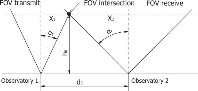
The field of view intersection of the transmit (observatory 1) and receive path (observatory 2) in bistatic configuration occurs at the height h0. The output diameter of the laser transmit telescope leads to a divergence angle αt. Separated by a distance d0, the field of view of the receive optics and the correlated angle αr is given by the focal length of the receive telescope and the size of the detector. If the intersection height of the field of views is higher than the region the atmospheric laser backscatter is originating from, no backscatter from the laser from observatory 1 can reach the received optics from observatory 2.

a Field of view intersection height h0 of transmit and receive system (separated by the distance d0) in dependence of the elevation ϵ. The telescopes point into the direction connecting both systems (azimuth ϕ = 0° or phi = 180°) which is the scenario with largest backscatter. The dashed blue line corresponds to the effective atmospheric backscatter height he, marking the estimate observation threshold. b, c Field of view intersection h0 in dependence of the azimuth ϕ and elevation ϵ for d0 = 4 m and d0 = 10 m. If at a given elevation h0 is lower than he, backscatter from the laser can enter the receiving system. The dashed blue line marks this threshold.
Noise filtering
To reduce the noise during SLR measurements usually narrow-band filters are used. This is especially important during daytime operation to reduce the sky noise background at wavelengths different from the laser wavelength. For the reduction of noise from the sunlight reflected by the satellite or the sky background two different filters with varying FWHM were tested: 1) Thorlabs, FWHM = 1.0 nm and 2) Alluxa, FWHM = 0.19 nm. For the Alluxa filter, a central filter wavelength above the nominal wavelength of the laser is chosen, as tilting the filter decreases the central wavelength. By gradually tilting the filter mounted in a COTS high-precision kinematic mount it is then possible to optimize the system to the nominal laser wavelength of 532.15 nm. The filter was also temperature-stabilized to within 0.5 °C to avoid any necessary re-adjustment of the filter, by connecting an oven via a proportional integral-derivative (PID) controller. Directly comparing the noise level for 22 recorded passes at 100 kHz showed a reduction of noise level by a factor of 4 when using the narrow-band filter.
MHz post-processing
Post-processing MHz laser ranging data can be a computationally demanding process if millions of data points are involved. For LEO satellites, data has to be read from files with sizes up to 1 GB. To accelerate read in times, Graz data format was converted to Apache Parquet. The column-based file format accelerated read in times by a factor of 20. For the calculation of Observed-Minus-Calculated (O-C) residuals, for each of the measured ranges data, a predicted range has to be calculated based on the reference orbit. This involves Lagrange interpolation and a conversion from X, Y, Z coordinates to local azimuth, elevation, and range. These two routines, though intrinsically simple, were found to be the main bottleneck during data analysis of large datasets. Speed issues were circumvented by using GPU-based programming, CUDA, and C++ code within the core Python-based cleaning program. With a single RTX3060 graphics card, when compared to Python (using vectorized functions) the GPU-based routines lead to an acceleration by a factor up to 25. The interpolation of x, y and z coordinates of 50 million points took 13.1 s with vectorized Python and only 0.5 s with GPU acceleration. As each variation of the reference orbit during post-processing involves the above mentioned transformation this step was crucial for efficiently reducing the data.
Read our previous article: ‘Raat Din Iske Peeche Lage Rahe’: Father Reveals How Yuvraj Singh Played Key Role In Abhishek Sharma’s Rise
Sports Update: . Stay tuned for more updates on Space debris and satellite laser ranging combined using a megahertz system and other trending sports news!
Your Thoughts Matter! What’s your opinion on Space debris and satellite laser ranging combined using a megahertz system? Share your thoughts in the comments below and join the discussion!