In what follows we provide additional details on a number of aspects of our analysis that we have omitted in the main text for compactness. These refer to the approach followed for the selection of the golden EOSs, the numerical techniques employed to simulate the binaries and extract the GW signal, and a number of validations highlighting the robustness of the correlation found between the EOS and the long-ringdown slope.
Selection of the golden EOSs
For the agnostic construction of cold EOSs, we begin from the GP setup presented in15, which we briefly review here. Below densities of n = 0.57 nsat, we use the crust model by Baym, Pethick, and Sutherland35; note that the uncertainty associated with the crustal EOS has been recently discussed in36. Above this density, in the interval n = [0.57, 10] nsat, a GP regression is performed in an auxiliary variable \(\phi (n):=-\ln (1/{c}_{s}^{2}(n)-1)\), where cs is the sound speed, and where the prior for ϕ(n) is drawn from a multivariate Gaussian distribution
$$\phi (n) \sim {{{\mathcal{N}}}}\left(-\ln \left(1/{\bar{c}}_{s}^{2}-1\right),K(n,{n}^{{\prime} })\right)\,,$$
(3)
with a Gaussian kernel \(K(n,{n}^{{\prime} })=\eta \exp (-{(n-{n}^{{\prime} })}^{2}/2{\ell }^{2})\)15. The hyper-parameters η, ℓ, and \({\bar{c}}_{s}^{2}\) within these definitions are themselves drawn from probability distributions
$$ \eta \sim {{{\mathcal{N}}}}\left(1.25,0.2{5}^{2}\right)\,,\quad \ell \sim {{{\mathcal{N}}}}\left(1.0\,{n}_{{{{\rm{sat}}}}},{(0.2{n}_{{{{\rm{sat}}}}})}^{2}\right)\,,\quad \\ {\bar{c}}_{s}^{2} \sim {{{\mathcal{N}}}}\left(0.5,0.2{5}^{2}\right)\,.$$
(4)
Below a density of 1.1 nsat, the GP is conditioned with the CEFT results from37. In particular, the average between the soft and stiff results from that work are taken as the mean, while the difference between them is taken as the 90% credible interval for the conditioning15. From this GP, we draw sample of 120,000 EOSs.
We impose the astrophysical observations referred to as Pulsars + \(\tilde{\Lambda }\) in15. Explicitly, we use the following three sets of observations:
-
1.
heavy-pulsar mass constraints from radio astronomy. In particular, we use the constraints from PSR J0348 + 0432 with M = 2.01 ± 0.04 M⊙38 and PSR J1624 − 2230 with M = 1.928 ± 0.017 M⊙39. We approximate the uncertainties from these measurements as normal distributions, which holds to good accuracy.
-
2.
joint tidal-deformability and mass-ratio constraints from GW observations. We use the two-dimensional (2D) joint probability distribution for the tidal deformability and mass ratio using the PhenomPNRT waveform model with low-spin priors from Fig. 12 of ref. 40.
-
3.
joint mass-radius measurements from X-ray pulse profile modeling. We use the 2D joint probability distribution for the mass and radius for PSR J0740 + 6620 using the NICER + XMM-Newton data from the right panel of Fig. 1 of ref. 41.
Within each of these measurements, we assume as our mass prior P0(M∣EOS) a uniform distribution between 0.5 M⊙ and MTOV.
Lastly, the GP is conditioned using information from high-density perturbative QCD calculations, which are under theoretical control at densities with baryon number chemical potential μ = 2.6 GeV, corresponding to n approximately 40nsat. This information is included in a conservative way, excluding those EOSs which cannot be connected to the perturbative densities using any causal, mechanically stable, and thermodynamically consistent interpolation in the density interval [10, 40] nsat42. This is done by conditioning the GP with the QCD likelihood function of ref. 15, where the uncertainty in the pQCD calculation at μ = 2.6 GeV is taken into account by marginalizing over the unphysical renormalization scale X: = 2Σ/(3μ) in the range [0.5, 2], with Σ the renormalization scale in the modified minimal subtraction scheme.
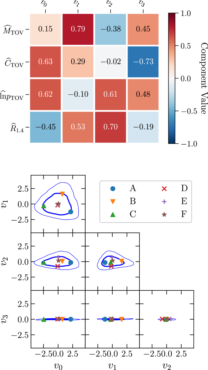
We consider the posterior in the 4D space of \(({M}_{{{{\rm{TOV}}}}},\,{C}_{{{{\rm{TOV}}}}},\,\ln {p}_{{{{\rm{TOV}}}}},\,{R}_{1.4})\), within which we perform a modified principal-component analysis to select a small sample of EOSs that characterize the 68% credible region of the distribution. This is done as follows:
-
1.
construct a normalized set of variables defined by \(\widehat{x}:=(x-{\mu }_{x})/{\sigma }_{x}\), with μx, σx the mean and standard deviation for the variable x.
-
2.
construct the 4 × 4 covariance matrix of these normalized variables.
-
3.
calculate the eigenvalues λi and eigenvectors vi of this covariance matrix, ordered by the magnitude on the eigenvalues.
The orthogonal vectors vi define the principal components of the distribution in the original 4D space, while the λi characterize the variance of the distribution in each of these directions. In principle, one could generalize this analysis by considering additional uncorrelated variables to the four we have chosen, or even attempt to identify the optimal set of uncorrelated variables, but this is beyond the scope of this work.
Figure 5 shows on the top panel the components vi in the normalized coordinate system, while the bottom panel shows the posterior distribution in the vi coordinate system.
Left panel: Components of the principal-component vectors vi in terms of the original (normalized) coordinates \(({\widehat{M}}_{{{{\rm{TOV}}}}},{\widehat{C}}_{{{{\rm{TOV}}}}},\widehat{\ln }{p}_{{{{\rm{TOV}}}}},{\widehat{R}}_{1.4})\). Bottom panel: Posterior distribution in the principle component analysis (PCA) coordinate system. Shown are 95% (thin lines) and 68% (thick lines) credible regions. Also shown are the six golden EOSs, with A–E lying on the 68% contour by construction, and F lying at the center. Source data for this figure are provided as a Source Data file.
As seen in this figure, the distribution is primarily 3D, with a prominent triangular component within the plane spanned by the components v0 and v1. This behaviour of the distribution clearly explains a well-known aspect to anyone constructing agnostic models of EOSs, namely, that while it is reasonable to model the variation in EOSs in terms of stiffness, i.e., \({\widehat{R}}_{1.4}\), this choice does not cover all of the possible space of parameters, which can be determined for instance in a principal-component analysis. Finally, we select the six golden EOSs from our ensemble by choosing EOSs that are near the extrema of the 68% credible region and one near the origin. With a standard principal-component analysis, these points would be given by \(\pm {\sqrt{\lambda }}_{i}{v}_{i}\) (no summation), which we modify slightly to capture the triangular shape within the plane spanned by v0 and v1. In this plane, we use the directions that extremizes the 95% credible regions. Having identified the relevant points in the parameter space, we then select the golden EOSs corresponding to one of these six points by finding the 30 closest EOSs using the Euclidean metric in the full 4D space and selecting the one with the highest likelihood. (For a short discussion of the robustness of this procedure, see SI note 1.) We note that using the reduced 3D metric obtained by dropping the v3 component leads to the same final golden EOSs. It is worth noting that using the corners of the 68% credibility contours for the golden EOS selection is a matter of choice in how we represent the underlying distribution. The variability of the simulations with the golden EOSs can be used as a proxy to approximate the 68%-credible regions that would be obtained if the full GP ensemble was used. In our analysis, this choice of 68% represents a compromise between capturing the extrema of the EOS distribution and assuring a sufficiently high posterior probability for the selected EOSs. In particular, choosing instead the 95% contour would represent the same distribution with a selection of EOSs coming from the tails of the EOS distribution, that is, EOSs that have significantly lower likelihood. This choice does not affect the overall results to the extent that our golden set characterises the features of the underlying distribution.
Merger simulations and GW analysis
The initial data for our simulations is generated using the spectral-solver code FUKA43, which allows us to produces both equal and unequal mass irrotational BNS initial configurations with an initial separation of approximately 45, km. FUKA employs the extended conformal thin-sandwich formulation of Einstein’s field equations to solve for binaries under the quasi-circular orbit approximation. Residual eccentricities are minimized by incorporating estimates for orbital and radial infall velocities at 3.5PN order43.
For the evolution, we employ the Einstein-Toolkit44, which incorporates the fixed-mesh box-in-box refinement framework Carpet45. Specifically, we utilize six refinement levels, with the finest grid having a spacing of 295, m, and impose reflection symmetry across the orbital plane. This resolution enables us to explore a reasonable portion of the EOS and BNS parameter space while maintaining manageable computational costs. The computational domain extends to an outer boundary at ± 1512, km, ensuring accurate gravitational wave extraction and appropriate boundary conditions.
For the spacetime evolution, we utilize Antelope46, a solver for the constraint-damping formulation of the Z4 system47. The evolution of matter is handled using the FIL general-relativistic magnetohydrodynamic code46, which employs fourth-order conservative finite-difference methods, ensuring high accuracy in hydrodynamic evolution even at the resolution adopted in this study. Additionally, FIL supports tabulated EOSs that depend on temperature and electron fraction and incorporates a neutrino transport scheme capable of modeling neutrino cooling and weak interactions48. To maintain our description as simple as reasonably possible, we have considered zero magnetic fields and neglected the radiative transfer of neutrinos; while we do not expect qualitative changes from either magnetic fields or neutrinos, it is reasonable to expect will play a quantitative role in establishing the long-ringdown slope.
As discussed in the main text, our agnostic EOS construction provides the cold (i.e., T = 0, where T is the temperature) part of the EOSs, while the thermal part is added during the evolution to account for shock-heating effects during and after the merger22. More specifically, the total pressure is given by the sum of the cold EOS pc = pc(ρ) and a thermal component pth = pth(ρ, T) = ρT, where ρ: = mBn is the rest-mass density and mB = 931.5 MeV the atomic mass unit. Analogously, the total specific internal energy can be separated into a cold ϵc = ϵc(ρ) and a thermal part ϵth = ϵth(T). Here, ϵc(ρ) = ec(ρ)/ρ–1 and ϵth(T): = T/(Γth–1), where ec(ρ) is the energy density of the cold EOS and Γth is the thermal adiabatic index, which we choose to take the constant value Γth = 1.75. As a result, the total pressure and total internal energy density are given by
$$p(\rho,T)={p}_{c}(\rho )+\rho T\,,\qquad \epsilon ( \, \rho,T)=\frac{{e}_{c}( \, \rho )}{\rho }-1+\frac{T}{{\Gamma }_{{{{\rm{th}}}}}-1}\,,$$
(5)
where the cold contributions ec(ρ) and pc(ρ) are provided in tabulated form by the GP construction explained above. The entropy can then be expressed as
$$s(\, \rho,T)=\frac{1}{{\Gamma }_{{{{\rm{th}}}}}-1}{{{\rm{\ln }}}}\left(\frac{{\bar{\epsilon }}_{{{{\rm{th}}}}}}{{\rho }^{{\Gamma }_{{{{\rm{th}}}}}-1}}\right)\,,$$
(6)
where \({\bar{\epsilon }}_{{{{\rm{th}}}}}:=\max ({\epsilon }_{{{{\rm{th}}}}},{s}_{{{{\rm{m}}}}in})\), with some numeric lower bound for the entropy smin = 10−10. In summary, our construction realizes a model-independent parametrization for the density and temperature dependence of viable NS EOSs without any information on the particle composition. Furthermore, since we neglect neutrino emission and absorption, no composition dependence is present in our simulations. Future analyses with self-consistent temperature-dependent EOSs could additionally explore a possible dependence of the long-ringdown slope on composition.
For the GW analysis, we adopt the Newman-Penrose formalism, which relates the Weyl curvature scalar ψ4 to the second time derivative of the polarization amplitudes of the GW strain h+,×, as described in ref. 49
$${\ddot{h}}_{+}+i{\ddot{h}}_{\times }={\psi }_{4}:={\sum }_{\ell=2}^{\infty }{\sum }_{m=-\ell }^{m=\ell }{\psi }_{4}^{\ell,m}{{-2}^{Y}}_{\ell,m}\,,$$
(7)
where sYℓ,m(θ, ϕ) are spin-weighted spherical harmonics with a weight of s = −2. From our simulations, we extract the multipoles \({\psi }_{4}^{\ell,m}\) at a sampling rate of about 634 kHz from a spherical surface of approximately 574 km radius, centered at the origin of the computational domain. The extracted data is then extrapolated to the estimated luminosity distance of 40 Mpc, corresponding to the GW170817 event50. We fix the angular dependence of the spherical harmonics by adopting a viewing angle of θ = 15°, as inferred from the jet orientation of GW17081751, and set ϕ = 0° without loss of generality. Our analysis is restricted to the multipoles with ℓ ≤ 4, noting that the ℓ = ∣m∣ = 2 modes dominate the signal. The relative difference in the maximum gravitational wave amplitude, \(\sqrt{{h}_{+}^{2}+{h}_{\times }^{2}}\), when comparing results including multipoles up to ℓ ≤ 4 and only ℓ = 2, is less than 3%. All results are presented as functions of the retarded time t–tmer, where tmer is defined as the time corresponding to the global maximum of the gravitational wave amplitude.
A key quantity in our analysis is the instantaneous GW frequency, fGW, defined as
$${f \! \!}_{{{{\rm{GW}}}}}:=\frac{1}{2\pi }\frac{d\phi }{dt}\,,\qquad \phi :=\arctan \left(\frac{{h}_{\times }^{2,2}}{{h}_{+}^{2,2}}\right)\,.$$
(8)
The radiated power is given by the integral expression49
$${\dot{E}}_{{{{\rm{G}}}}W}=\frac{{r}^{2}}{16\pi }{\sum }_{\ell=2}^{\infty }{\sum }_{m=-\ell }^{\ell }{\left| \int_{ \! \! \! \! \! -\infty }^{t}d{t}^{{\prime} }{\psi }_{4}^{\ell m}\right| }^{2}\,,$$
(9)
where the total emitted GW energy follows from another time integration \({E}_{{{{\rm{GW}}}}}(t):=\int_{ \! \! -\infty }^{t}d{t}^{{\prime} }{\dot{E}}_{{{{\rm{GW}}}}}({t}^{{\prime} })\). Similarly, the rate of radiated angular momentum is defined as49
$${\dot{J}}_{{{{\rm{GW}}}}}:=\frac{{r}^{2}}{16\pi }{{{\rm{Im}}}}\left\{{\sum }_{\ell=2}^{\infty }{\sum }_{m=-\ell }^{\ell }m\left(\int_{ \! \! \! \! \! -\infty }^{t}d{t}^{{\prime} }{\psi }_{4}^{\ell m}\right)\int_{ \! \! \! \! \! -\infty }^{t}d{t}^{{\prime} }\int_{ \! \! \! \! \! -\infty }^{t{\prime} }d{t}^{{\prime\prime} }\,{\bar{\psi }}_{4}^{\ell m}\right\}\,,$$
(10)
where r is the observer distance and where \({\bar{\psi }}_{4}\) is the complex conjugate of ψ4 and the total emitted angular momentum follows again from another time integration \({J}_{{{{\rm{GW}}}}}(t):=\int_{ \! \! -\infty }^{t}d{t}^{{\prime} }{\dot{J}}_{{{{\rm{G}}}}W}({t}^{{\prime} })\).
In the main text we work with dimensionless energies \({E}_{{{{\rm{G}}}}W}(t)/{E}_{{{{\rm{GW}}}}}^{{{{\rm{mer}}}}}\) and angular momenta \({J}_{{{{\rm{GW}}}}}(t)/{J}_{{{{\rm{G}}}}W}^{{{{\rm{mer}}}}}\) obtained by normalizing with the respective values at merger time \({E}_{{{{\rm{GW}}}}}^{{{{\rm{mer}}}}}:={E}_{{{{\rm{GW}}}}}({t}_{{{{\rm{mer}}}}})\) and \({J}_{{{{\rm{G}}}}W}^{{{{\rm{mer}}}}}:={J}_{{{{\rm{GW}}}}}({t}_{{{{\rm{mer}}}}})\). When expressed in terms of strain components, and in full generality, the ratio of the radiated energy and angular-momentum rates dEGW/dJGW is similar to the instantaneous GW frequency
$$\frac{d{E}_{{{{\rm{GW}}}}}}{d{J}_{{{{\rm{GW}}}}}}=\frac{{\dot{E}}_{{{{\rm{GW}}}}}}{{\dot{J}}_{{{{\rm{G}}}}W}}=\frac{{\dot{h}}_{+}^{2}+{\dot{h}}_{\times }^{2}}{{h}_{+}{\dot{h}}_{\times }-{\dot{h}}_{+}{h}_{\times }}\,,\qquad {f}_{{{{\rm{GW}}}}}=\frac{1}{2\pi }\frac{{h}_{+}{\dot{h}}_{\times }-{\dot{h}}_{+}{h}_{\times }}{{h}_{+}^{2}+{h}_{\times }^{2}}\,.$$
(11)
For a simple system with an ℓ = 2, m = 2 deformation, e.g., a compact rotating system with eccentric mass distribution like the toy model of ref. 10 and for which \({h}_{+}(t)\propto \cos (\phi (t))\) and \({h}_{\times }(t)\propto \sin (\phi (t))\) with GW phase ϕ(t), one obtains the identity \({\dot{E}}_{{{{\rm{GW}}}}}/{\dot{J}}_{{{{\rm{GW}}}}}={f}_{{{{\rm{GW}}}}}/(2\pi )\). Since in the long ringdown \({f}_{{{{\rm{GW}}}}}(t)\simeq {{{\rm{const.}}}}=:{f}_{{{{\rm{rd}}}}}\), expressions (11) explain why the radiated energy and angular momentum are linearly related.
Finally, we analyze the spectral features of the waveforms and compute the PSD of the signal as10
$${\tilde{h}}^{\ell,m}(\, \, f):=\frac{1}{\sqrt{2}}{\left({\left| \int\,dt{{{{\rm{e}}}}}^{-2\pi ift}{h}_{+}^{\ell,m}(t)\right| }^{2}+{\left| \int\,dt{{{{\rm{e}}}}}^{-2\pi ift}{h}_{\times }^{\ell,m}(t)\right| }^{2}\right)}^{1/2}\,,$$
(12)
where the time integration is performed over the interval t–tmer ∈ [0, 30] ms or up to the time at which a black hole is formed if the post-merger remnant collapses earlier. As done routinely (see, e.g., refs. 9,10,11,12,14), the dominant post-merger frequency f2 is then determined by the global maximum of the PSD.
Read our previous article: 10 highest-graded Chiefs, Eagles players ahead of Super Bowl 59
Sports Update: 49$${\ddot{h}}_{+}+i{\ddot{h}}_{\times }={\psi }_{4}:={\sum }_{\ell=2}^{\infty }{\sum }_{m=-\ell }^{m=\ell }{\psi }_{4}^{\ell,m}{{-2}^{y}}_{\ell,m}\,,$$ (7) where syℓ,m(θ, ϕ) are spin-weighted spherical harmonics with a weight of s = −2 Stay tuned for more updates on Constraining the equation of state in neutron-star cores via the long-ringdown signal and other trending sports news!
Your Thoughts Matter! What’s your opinion on Constraining the equation of state in neutron-star cores via the long-ringdown signal? Share your thoughts in the comments below and join the discussion!