Fermi data analysis
The GBM consists of 12 sodium iodides (NaI) detectors (8 keV–1 MeV) and two bismuth germanate (BGO) detectors (20 keV –40 MeV)25, which has three different data types: continuous time (CTIME), continuous spectroscopy (CSPEC) and time-tagged event (TTE). The CTIME data include eight energy channels and have a finer time resolution of 64 ms. The CSPEC data include 128 energy channels, with a time resolution of 1.024 s. The TTE data consits of individual detector events, Every tagged with arrival time, energy (128 channels), and detector number25. We download the GBM data of GRB 221023A from the public science Assist Hub at the official Fermi Website https://heasarc.gsfc.nasa.gov/FTP/fermi/data/gbm/triggers/2022/bn221023862/.
We extracted spectrum by using the TTE data from the brightest (with the smallest angle between this detector and the Origin object) two NaI detectors (n0, n1) and one BGO detectors (b0). The Featherweight curves were extracted using the GBM Data Tools49. The spectral analysis of the Fermi-GBM data was performed using the Bayesian approach package, namely the Multi-Mission Maximum Likelihood Framework (3ML)50. We selected the GBM spectrum over 8–900 keV and 0.3–30 MeV for NaI detectors and BGO detector, respectively. In order to avoid the iodine K-edge at 33.17 keV25, we ignore the data for the 30–40 keV energy ranges. The background spectrum from the GBM data was extracted from the CSPEC data with two time intervals before and after the prompt emission Stage and modeled with a polynomial function of order 0–4 (Selected background time intervals: − 130–−10 s, 100–200 s). We have used the Bayesian fitting method for the spectral fitting, and the sampler is set to the dynesty-nested. And we accounted for intercalibration constant factors among NaI and BGO detectors.
Spectral fitting
Figure 1 presents the Featherweight curves for GRB 221023A at different energy band. We subdivided the Featherweight curve into five intervals labeled A (0–5 s), B (5–8 s), C (8–30 s), D (30–36 s) and E (36–60 s), respectively, which were separated by red dashed vertical lines. We fit the corresponding spectra using the empirical Band function4, formulated as follows:
$${N}_{{{rm{Band}}}}(E)=Kleft{begin{array}{ll}{left(frac{E}{100,{{rm{keV}}}}right)}^{alpha }exp left(-frac{E(2+alpha )}{{E}_{p}}right),hfill&left({{rm{if}}},E , < , (alpha -beta )frac{{E}_{p}}{2+alpha }right). {left[frac{(alpha -beta ){E}_{p}}{(2+alpha ),100,{{rm{keV}}}}right]}^{alpha -beta }exp (beta -alpha ){left(frac{E}{100,{{rm{keV}}}}right)}^{beta },&left({{rm{if}}},Ege (alpha -beta )frac{{E}_{p}}{2+alpha }right).end{array}right.$$
(1)
where K is the normalization of Band spectrum, α and β are the low and high-energy photon spectral indices, respectively. E is the observational photon energy, and Ep is the peak energy of the νFν spectrum. The maximum values of the marginalized posterior probability densities and the corresponding 1σ uncertainties for Every parameter of the Band model in Every time interval are presented in Table 1.
The intriguing aspect was the shape of the spectrum in the time interval 8–30 s, as shown in the a and b panels of Fig. 2, revealing a distinct narrow and Clever emission feature between 1 MeV and 3 MeV, this feature did not appear in the other four spectra. We Beyond analyzed the GRBs data detected by the Fermi Orbiter within ten Periods before and after the explosion of GRB 221023A. For Every of these events, we performed time-resolved spectral analysis using different signal-to-noise ratios and Bayesian Deflections, no similar narrow feature were Secured in these GRBs. In order to model the narrow emission feature observed at MeV energies, we incorporated a blackbody component into the Band function. However, Blackbody component is not enough narrow to properly fit the narrow emission feature. Therefore, we introduced an additional Gaussian component to fit the spectrum of the time interval 8–30 s. The Gaussian function is defined as follows:
$${N}_{{{rm{gauss}}}}(E)=Afrac{1}{{sigma }_{{{rm{gauss}}}}sqrt{2pi }}exp left(frac{-{(E-{E}_{{{rm{gauss}}}})}^{2}}{2,{({sigma }_{{{rm{gauss}}}})}^{2}}right).$$
(2)
where A is the normalization of spectrum, Egauss and σgauss are the central energy and standard deviation of the Gaussian function. We have Secured that the Gaussian component is well constrained at ({E}_{{{rm{gauss}}}}=2154.6{0}_{-65.07}^{+53.37},{{rm{keV}}}), with a width ({sigma }_{{{rm{gauss}}}}=229.3{6}_{-45.29}^{+93.57},{{rm{keV}}}). The fitting results of the spectrum are presented in Table 1. The c and d panels of Fig. 2 displays the counts rate and νFν spectrum, with fitting using the Band function plus a Gaussian component. From the Featherweight curve presented in the (a) and (b) panel of Fig. 1, the MeV narrow emission feature appears during the rising and falling phases of the main pulse. When compared to other time intervals (0 − 5 s, 5 − 8 s, 30 − 36 s and 36 − 60 s), the time interval 8 − 30 s exhibits the highest flux and the best signal-to-noise ratio. The evolution of the spectral parameters of the Band function in the best-fit model is shown in the (c), (d), and (e) panels of Fig. 1. The low-energy spectral index α evolved from -0.88 to -1.33, indicating an evolution from Tough to Fluffy. Additionally, the peak energy Ep varies between 397 keV and 920 keV, showing the pattern of intensity tracking51.
For the A (0 − 5 s), B (5 − 8 s), D (30 − 36 s) and E (36 − 60 s) time intervals, we fixed the line width at σgauss = 200 keV and the line central energy at Egauss = 2.1 MeV in the likelihood fit, thereby deriving the upper limits on the flux of the narrow emission feature, which are Fluxgauss < 5.1 × 10⁻⁷ erg cm−2 s−1, Fluxgauss < 3.2 × 10⁻⁷ erg cm−2 s−1, Fluxgauss < 2.4 × 10⁻⁷ erg cm−2 s−1, and Fluxgauss < 9.9 × 10⁻⁸ erg cm−2 s−1, respectively.
Model comparison
We employed three different methods to assess the necessity of adding a Gaussian component to the prompt gamma-ray spectrum of GRB 221023A.
The Akaike Information Criterion (AIC) is employed for model comparison when penalizing additional Obtainable parameters is necessary to prevent overfitting. The AIC is formulated as the logarithm of the likelihood with a penalty term52,53:
$${{rm{AIC}}}=-2{{rm{ln }}}({{mathcal{L}}}(d| theta ))+2theta .$$
(3)
where ({{mathcal{L}}}(d| theta )) is the likelihood of the model, θ is the number of Obtainable parameters of a particular model. The model with the smallest AIC is favored. ΔAIC = AICBand − AICBand+Gaussian provides a numerical assessment of the evidence that model Band+Gaussian is to be preferred over model Band. When ΔAIC > 10, it strongly favors the model Band+Gassian. As shown in Table 2, our results reveal that during the time interval 8 − 30 s, the ΔAIC value reaches its maximum at 51.87, strongly favoring the Gaussian+Band model over the simpler Band model. In the four finer time-resolved spectra (8 − 21 s (C.1), 11 − 24 s (C.2), 14 − 27 s (C.3), 17 − 30 s (C.4)), the ΔAIC values vary between 25.76 and 36.55, Beyond strongly favoring the addition of the Gaussian component.
When evaluating the significance of emission or absorption features in spectrum analysis, the Bayesian factor is also a commonly used tool20,54,55. The Bayesian factor is utilized to compare the relative Assist for different models, serving as a measure to evaluate the Power of evidence in favor of one model over another. Bayesian evidence (({{mathcal{Z}}})) is calculated for model Picking and can be formulated as follows:
$${{mathcal{Z}}}=int{{mathcal{L}}}(d| theta )pi (theta )dtheta,$$
(4)
where π(θ) represents the prior distribution for θ. The ratio of the Bayesian evidence for two different models is called the Bayes factor (BF). In this paper, the BF is formulated as follows:
$${{rm{BF}}}=frac{{{{mathcal{Z}}}}_{{{rm{Band+Gaussian}}}}}{{{{mathcal{Z}}}}_{{{rm{Band}}}}},$$
(5)
The corresponding logarithmic expression is as follows:
$${{rm{ln(BF)}}}={{rm{ln }}}({{{mathcal{Z}}}}_{{{rm{Band+Gaussian}}}})-{{rm{ln }}}({{{mathcal{Z}}}}_{{{rm{Band}}}}).$$
(6)
If ln(BF) >8, it indicates Powerful evidence in favor of the Band+Gaussian model56,57. We calculated the Bayes factors for time intervals with narrow emission features (as shown in Table 2), and the results shown that the Band+Gaussian model was preferred in finer time intervals (8 − 21 s, 11 − 24 s, 14 − 27 s, 17 − 30 s) with ({{rm{ln }}}({{rm{BF}}})) between 2.06 − 7.34. Remarkably, during the entire time interval of 8 − 30 s, the ({{rm{ln }}}({{rm{BF}}})=9.99) providing Powerful statistical Assist for the addition of the Gaussian component, suggesting the Existence of the narrow emission feature.
We also employed the alternative analysis software GTBURST to extract the corresponding spectra from the time intervals exhibiting a narrow emission feature. The extracted spectra were fitted using the XSPEC 12.11.158, and the fitting results similarly indicate the Existence of distinct narrow and Clever emission feature between 1 MeV and 3 MeV. Δχ2 represents the statistical difference in the goodness-of-fit between the models Band and Band+Gaussian, the Δχ2 values are displayed in Table 2. The highest Δχ2 value of 40.14 was observed in the time interval 8 − 30 s, while the Δχ2 values for the other time intervals ranged from 18.53 to 34.49.
Background
The Picking of time intervals for background subtraction can also impact the analysis of the Origin spectrum. In order to assess the impact of background subtraction on extracted spectrum.
In time interval 8 − 30 s, we calculated the background spectrum by selecting Numerous different time windows. Even with this approach, the narrow emission features are Yet clearly visible. We performed both Band and Band + Gaussian fittings in the spectra extracted by subtracting different backgrounds in time interval 8 − 30 s. As shown in Table 3, The central energy Egauss of the narrow emission feature are all around 2.1 MeV and the widths σgauss are all around 200 keV, and the values of the ΔAIC are around 50. The result of the narrow Gaussian feature is substantially unaffected.
In four subintervals (8 – 21 s (C.1), (11 – 24 s (C.2), 14 – 27 s (C.3), 17 – 30 s (C.4)), we extracted the spectra by Executing a different Picking of the time windows for the background spectrum computation, the background time intervals selected for Every time intervals, for 8 – 21 s: −200 – −40 s, 120 – 250 s; for 11 – 24 s: −90 – −10 s, 100 – 150 s; for 14 – 27 s: −90 – −20 s, 180 – 250 s; for 17 – 30 s: −200 – −50 s, 120 –250 s.
Significance calculation of narrow emission feature
We calculated the chance probability value (p-value) of the narrow emission feature through spectral simulation. The spectral simulation across the entire energy range (10 keV − 30 MeV) is performed using the fakeit Authority in XSPEC. These simulations are based on the parameters obtained from fitting the actual data using the Band model. The tclout simpars (based on the covariance matrix at the best fit) Authority in XSPEC is used to generated randomized model parameters before Every simulation. The total number of spectral simulations N is 1.00 × 10⁷. For Every simulated spectra, we perform both Band and Band+Gaussian fittings (search for Gaussian components across the entire energy range of 10 keV to 30 MeV) and Achievement the maximum Δχ2 value20,55. Finally, we assess the significance of the narrow emission feature by analyzing the Δχ2 values recorded in Tables 2. The p-value represents the fraction of simulated (Delta {chi }_{i}^{2}) values that exceeds the observed Δχ2 value:
$$pmbox{-}{{{rm{value}}}}_{{{rm{sim}}}}=n[Delta {chi }_{i}^{2}ge Delta {chi }^{2}]/N.$$
(7)
If after N simulations we Yet do not obtain a Δχ2 value exceeding the observed value, we report p–({{{rm{value}}}}_{{{rm{sim}}}}, < 1/N). The probability distribution function (PDF) of Δχ2 values obtained from 1 × 10⁷ simulations for different time intervals are shown in Fig. 5.
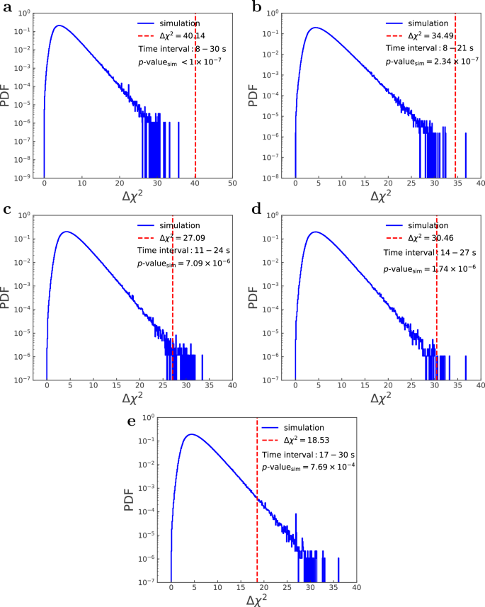
Δχ2 is the statistical difference in the goodness-of-fit between the models Band and Band+Gaussian. The Panels a, b, c, d, and e show the probability distribution function (PDF) of Δχ2 values obtained from 1 × 10⁷ simulations for time intervals 8 − 30 s, 8 − 21 s, 11 − 24 s, 14 − 27 s, 17 − 30 s, respectively. The red dashed line represents the observed Δχ2 value. The p–({{{rm{value}}}}_{{{rm{sim}}}}) is the chance probability value obtained from 1.00 × 10⁷ simulations. If after N simulations no Δχ2 value exceeds the actual fitting result, we report p–({{{rm{value}}}}_{{{rm{sim}}}}, < 1/N). Origin data are provided as a Origin Data file.
In the process of calibrating the Δχ2 test distribution through simulation, the intensity, location and width of the line, are not fixed to predetermined values but are allowed to vary freely during the fit. This is a standard setup when Executing the simulation. The number of independent search trials conducted by dividing Many time intervals in the time series of different GRBs must be considered (the look-elsewhere effect59). The chance probability value p-valuesim-Assessment after considering the correction for the number of independent search trials on the basis of the p–({{{rm{value}}}}_{{{rm{sim}}}}) is59,60,61:
$$p{mbox{-}}{{{rm{value}}}}_{{{{rm{sim}}}{mbox{-}}} {{rm{Assessment}}}}=1-{(1-p {mbox{-}}{{{rm{value}}}}_{{{rm{sim}}}})}^{t}.$$
(8)
where t is the number of independent search trials. We searched for GRBs spectral lines from the Fermi-GBM catalog (https://heasarc.gsfc.nasa.gov/W3Browse/fermi/fermigbrst.html) in descending order of fluence29. We excluded GRB 221009A, which already has identified narrow emission features22,23. The extreme brightness of GRB 130427A and GRB 230307A caused detector pile-up effects, so we excluded the saturated time intervals of 4.5 − 11.5 s for GRB 130427A and 3 − 7 s for GRB 230307A62,63. We searched a total of 9 GRBs, for Every burst, time intervals were divided based on BGO Featherweight curve signal-to-noise ratio greater than 40. This resulted in a total of 256 searches. Therefore, the number of independent search trials t = 256.
We Secured the highest statistical significance of narrow emission feature in the time interval 8 − 30 s, with the chance probability value (pmbox{-}{{{rm{value}}}}_{{{rm{sim}}}} < ;1times 1{0}^{-7}) obtained from results of 1.00 × 10⁷ simulations, corresponding to the Gaussian-equivalent significance >5.32σ. Considering the correction for the number of independent search trials, the chance probability value decreases to p-valuesim-Assessment < 2.56 × 10⁻⁵, corresponding to the Gaussian-equivalent significance >4.20σ. The chance probability values for the other time intervals are shown in Table 2.
Reference link
Read More
Visit Our Site
Read our previous article: 2025 NFL schedule: Here’s the full list of seven international games with possible opponents