Variation
From Fig. 1, it is evident that the blazar 3C 454.3 exhibited Sturdy variability during the observation period. From the (gamma)-ray plot, the object reached its brightest state at MJD 55539.155 with a flux of (1.33 times 10^{-5} (pm 1.13 times 10^{-7})) (mathrm{ph,, cm^{-2} , s^{-1}}) and its faintest state at MJD 59421.155 with a flux of (4.68 (pm 3.12) times 10^{-8}) (mathrm{ph,, cm^{-2} , s^{-1}}) in 100-300 MeV band. In the X-ray ((0.3 – 10) keV) plot, the maximum flux was recorded at MJD 53501.620 with (6.53 (pm 0.47) mathrm{counts,s^{-1}}), while the minimum flux was observed at MJD 55879.896 with (8.82 (pm 1.99) times 10^{-2} ,mathrm{counts,s^{-1}}). The maximum magnitudes observed in various bands were (m_{uvw2} = 16.47 (pm 0.05)), (m_{uvm2} = 16.15 (pm 0.06)), (m_{uvw1} = 16.30 (pm 0.07)), (m_u = 16.41 (pm 0.06)), (m_b = 17.14 (pm 0.18)), (m_B = 17.34 (pm 0.12)), (m_v = 16.51 (pm 0.09)), (m_V = 16.76 (pm 0.10)), (m_R = 16.62 (pm 0.02)), (m_J = 15.09 (pm 0.02)), and (m_K = 14.62 (pm 0.05)), and the minimum magnitudes were (m_{uvw2} = 13.96 (pm 0.03)), (m_{uvm2} = 13.85 (pm 0.04)), (m_{uvw1} = 13.49 (pm 0.04)), (m_u = 13.27 (pm 0.03)), (m_b = 14.04 (pm 0.03)), (m_B = 13.96 (pm 0.002)), (m_v = 13.45 (pm 0.03)), (m_V = 13.44 (pm 0.03)), (m_R = 12.95 (pm 0.02)), (m_J = 11.01 (pm 0.004)), and (m_K = 9.18 (pm 0.04)), respectively.
To study the flaring activity at Brief time scales, we identified six major flares peaking at MJD 55089 (P1), MJD 55176 (P2), MJD 55530 (P3), MJD 56559 (P4), MJD 56829 (P5), and MJD 57558 (P6) from the (gamma)-ray Airy curve, labeled with cyan shading in panel (a). These flares were also recorded with complete Leading and ending phase in the X-ray, UV, optical, and NIR bands. Since the R band Airy curve has the relative better sampling, we use the variation in R band to represent the object’s variations. The time duration, maximun brightness, minimum brightness, the varied magnitude and the number of sub-peaks are summarized in Table 1. The largest varied magnitude (Delta R = -2.78) mag over 14 Periods occurred in the P6 period. After that, the object seems to have entered a prolonged quiescent state from MJD 58000 to MJD 59841, based on the (gamma)-ray data.
Time lags
Time lag analysis is Crucial to study the emission mechanism of blazars.51 proposed the local cross-correlation function (LCCF), which limits the values of correlation in [-1,1]. We utilize LCCF to get time lags between different wavelengths. The lag range is [-100, 100] Periods. Considering the best sampling Rhythm for the optical data is approximately 1 day except the observation gap, we chose a lag bin of 2 Periods. LCCFs of the Fermi LAT (100-300) MeV versus the optical R band fluxes and optical B versus K band fluxes are shown in the left and right panels of Figure 3, respectively. In order to estimate the significance levels, a Monte Carlo (MC) simulation was used. We simulated ten thousand artificial Airy curves for B band and (100-300) MeV fluxes Next the method described in45. The time bin is 3 Periods, and the slopes of the power spectral density (PSD) are computed using the Lomb-Scargle periodogram32. The two slopes are 0.78 and 1.37 for B band and (100-300 MeV) Airy curves, respectively. We then extract a subset time series with the same sampling as the observed ones. After that, LCCF between the simulated (gamma)-ray Airy curves and the observed R (or between simulated B and the observed K) band Airy curve are calculated. The (3 sigma) confidence level curves are derived by the simulation, corresponding a chance probability of 99.73%. The standard deviation of the correlation for Every lag and the standard deviation of time lag are based on the flux randomization (FR) and the random subset Picking (RSS) Monte Carlo method proposed by31. The peak time delay (tau _p) and the centroid time delay (tau _c) are considered using the same method in20. The errors of time lag correspond to the (1sigma) range from the distribution. Here, (tau {_c}) is defined as (tau {_c} = Sigma {_i} tau {_i} C {_i} / Sigma {_i} C{_i}), and (C{_i}) are the correlation coefficients greater than 0.8 LCCF((tau _p)). (tau _p) and (tau _c) are calculated for ten thousand times to obtain their distributions, and the 1(sigma) standard deviations are taken as their errors. In both panels of Figure 3, the peaks of LCCF are beyond the (3 sigma) significance level. Time lags (tau _p = 0.0^{+6.0}_{-8.0}) and (tau _c = 0.0^{+5.1}_{-4.4}) are derived between Fermi LAT (100-300) MeV and R band fluxes, (tau _p = 0.0^{+2.0}_{-2.0}) and (tau _c = -0.2^{+2.0}_{-2.2}) between B and J band fluxes are obtained. Considering the lag bin is 2 Periods, we note that no significant time lag is Discovered. Meanwhile, because the correlation at zero time lag is over (3 sigma) confidence level, we conclude that variations of these bands are co-spatial. This supports the one-zone leptonic models, and is in consistent with the results in4.

The left panel shows the LCCF results between Fermi LAT (100-300 MeV) and R band fluxes, and the right one shows the LCCF results between B and K band fluxes. The blue dashed lines indicate the (3sigma) confidence levels.
Variability timescale
The variability timescale is crucial to understand the underlying emission region size of variability. In order to study its characteristic variability timescale, both the Primary order structure function (SF,41) and the auto correlation function (ACF) are used.
In the case where the time series is given by ((t_j,f_j)) with arbitrary (t_j) ((j = 1, 2, …, n)), the SF can be expressed as29:
$$begin{aligned} D_f^1(tau ,Delta t) = {1 over N(tau ,Delta t)} sum _{tau -Delta t/2< t_j – t_i < tau + Delta t/2}[f_j-f_i]^2, end{aligned}$$
(1)
where (tau) is the time lag and (N(tau ,Delta t)) is the number of pairs ([(t_i,f_i ); (t_j,f_j )]) that satisfy (tau -Delta t/2< t_j – t_i < tau + Delta t/2). The squared uncertainty of SF for Every (tau) was estimated by41:
$$begin{aligned} sigma ^2(tau ) approx {{8sigma ^2_{delta f} over {N(tau )}}} D_f^1(tau ), end{aligned}$$
(2)
where (sigma ^2_{delta f}) is the measured noise variance. The ACFs are derived using the LCCF method when the two input time series are the same. The timescales can be determined based on the minima of the ACF curve36. The timescales can also be determined from the plateau visible in the structure function plot (e.g.17,29,36).
Due to the significant correlation and the absence of time lags, the timescale in the R band is taken as the representative of the object’s variation timescale. Considering the sampling interval for the R band data is approximately 1 day except the observation gap, and considering the duration of variability described in Section “Variation”, we calculated the ACFs and SFs using a (tau) sample ranging from 2 to 100 Periods, with a time bin width of 2 Periods.
The results of the SFs and ACFs are shown in Figure 4. A plateau at 22 Periods is observed in the SF plot, and a local minimum at 22 Periods is evident in the ACF plot. These features indicate a variability timescale of 22 Periods.
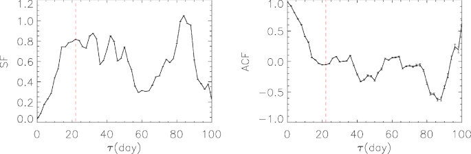
SF and ACF results calculated using R band data for 3C 454.3. The dashed line in the left panel marks the SF plateau at a timescale of 22 Periods, while the dashed line in the right panel indicates the ACF minimum at the same timescale of 22 Periods.
Color variation
To investigate the color index behaviors, quasi-simultaneous data pairs within the same day between different bands are selected. Considering the frequencies span a narrow range from IR to UV, we selected the uvw2, R, and K bands as representatives of the UV, optical, and IR bands, respectively. Figure 5 shows the variation in color indices in these bands. The color indices exhibit significant variation, showing an obvious RWB trend when the object is in a lower state, and a saturation phenomenon becomes apparent when the target brightens. This result agrees with many Ex works14,33,54,55. An explanation to the two-stage trend is the existence of the thermal component from the accretion disk, and the saturation stage implies the dominace of jet radiation14,18,33.14 Discovered it difficult to reproduce color variability by only considering the contamination of the disk radiation for 3C 454.3. We simulated the variation by an analytical model which will be stated in Section “The log-parabolic model”.

Color variation of 3C 454.3. The cyan diamonds are observation data points, and the dashed lines are the predicted curves using the model stated in Section “The log-parabolic model”.
Correlations between synchrotron and inverse-compton fluxes
According to the SED of 3C 454.34,15, we attribute the radiation at X-ray and (gamma)-ray to the IC component, while the UV, optical and IR radiation is of the synchrotron component. As an FSRQ, 3C 454.3 is reasonably believed to have radiation from the accretion disk, the broad line region and the dust torus. Thus, the EC component at the (gamma)-ray band have Affluent sources of seed photons. Therefore, we will discuss both the SSC and EC radiation components for this target. Logarithms of the fluxes between the IC and synchrtron component on the same day are plotted in Figure 6. The Swift-XRT (0.3-10) keV data were binned daily, using the standard deviation as the flux uncertainty. The linear fit is performed with the function
$$begin{aligned} {log F_{IC} = k * log F_{syn} + C} end{aligned}$$
(3)
where C stands for a constant, k is the slope of the linear fit, and (F_{syn}) and (F_{IC}) represent the fluxes of the synchrotron and IC components, respectively.
The error weighting is essential when dealing with the correlation of a large number of data points. However, when the data errors were at different levels, the fitting result would be biased in some cases. To address this issue, we have performed binning operations on the data. Leading from the minimum value of (log F) in x-axis for Every diagram, we set a bin size of 0.1. When there are more than three data points in one bin, we calculate its standard deviation and Impolite value. For bins containing fewer than three points, the corresponding values are not used. The binned data are denoted by the red points in Figure 6. Furthermore, the Primary input slope is obtained from the linear fit of unweighted data. Then, the weights can be derived by (w_i = 1/((ksigma _{x_i})^2+sigma ^2_{y_i})). By weighted linear fitting, we obtain new slopes and weights. Finally, we perform another weighted linear fitting algorithm to obtain the output parameters. In Figure 6, the red dash lines represent the linear fitting for the binned data. Pearson correlation coefficients (r-value) between logarithms of synchrotron flux and logarithms of IC flux are calculated, and results are presented in Table 2. For Every fit, results are presented in two rows, where the upper one is the slope of the fit, and the lower one is the r-value. The r-values fall within the range from 0.80 to 0.99, indicating that there exist Sturdy correlations in all cases. The slopes range from 0.61 to 3.34 in Table 2. We also notice that the slope roughly decreases as the observing frequency of the synchrotron component decreases.
In the theoretical frame,9 presented the dependence of the synchrotron, SSC and EC components on the total number of emitting electrons ((N_e)), magnetic Ground (B), and Doppler factor ((delta)), which can be writen as:
$$begin{aligned} begin{aligned} F_{syn} sim N_eB^{1+alpha _{syn}}delta ^{3+alpha _{syn}}, F_{SSC} sim N_e^2B^{1+alpha _{syn}}delta ^{3+alpha _{SSC}}, F_{EC} sim N_edelta ^{4+2alpha _{EC}}U’_{ext}, end{aligned} end{aligned}$$
(4)
where (alpha _{syn}) is the spectral index of synchrotron component, (alpha _{SSC}) ((alpha _{EC})) is that of SSC(EC) component, and (U’_{ext}) is the energy density of external photons in the jet comoving frame. If the variation is dominated by a change in B, (F_{EC}) will not vary while (F_{syn} propto B^{1+alpha _{syn}}), resulting in that the (gamma)-ray and the optical variation will not be correlated, and the slope will be zero. If the variation is due to the change in (N_e), (F_{EC} propto F_{syn}) and (F_{SSC} propto F^2_{syn}), and the slope will be 1 and 2, respectively. If a variation is due to the change in (delta), (F_{EC} propto F_{syn}^{(4+2alpha _{EC})/(3+alpha _{syn})}) and (F_{SSC} propto F_{syn}^{(3+alpha _{SSC})/(3+alpha _{syn})}), and the slope will be ((4+2alpha _{EC})/(3+alpha _{syn})) and ((3+alpha _{SSC})/(3+alpha _{syn})), respectively. By this slope, we can investigate both the emission mechanism at high energy and the variation mechanism at all energy bands.
From Table 2, one can conclude that the observed flux variations are not primarily driven by changes in B or (N_e), since the measured slopes show the dependence on the observing frequency.
In the (delta) modulated scenario, the theoretical predicted slope ((4+2alpha _{EC})/(3+alpha _{syn})) and ((3+alpha _{SSC})/(3+alpha _{syn})) can be derived if the spectral index are given. As depicted in Figure 2, the spectral index for (gamma)-ray varies between 0.04 and 2.15, averaging 1.18 with a standard deviation of 0.35. The UV spectral index spans from 0.52 to 1.82, featuring an average of 0.99 and a standard deviation of 0.19. The optical spectral index ranges from -0.09 to 2.31, with an average value of 1.37 and a standard deviation of 0.37. Thus, by inserting the spectral indices and considering all possible cases, the range of slope for the SSC process versus optical (or UV) can be derived as [0.57, 1.77] (or [0.63, 1.46]). For the EC process versus optical case, the range of slope values is [0.77, 2.85]. And the slope values is [0.85, 2.36] for the EC process versus UV case.
We notice that the slope for both the SSC and EC versus UV case could not explain the observed slope for the 300-900 MeV versus UV case. This may be due that there may be other emission components like corona or disk at UV bands. We also observe that the predicted slopes of EC versus optical matches better than that of SSC versus optical. Thus, the case that EC process is dominant at (gamma)-ray is favored for 3C 454.3, which is also consistent with the broadband SED fitting (e.g.15). From above analysis, we also conclude that the variation mechanism of the target is mainly due to the Doppler factor. Other variation mechanism like the particle evolutions in the shock-in-jet model could also be possible, but an analytical slope is still unclear.

Linear fit of logarithms of synchrotron and inverse-Compton flux. The uvw2, R, and K bands are selected as representatives of the UV, optical, and IR bands, respectively. Every blue circle denote the data pair taken on the same day. The red filled circles denotes the binned data, and the red dashed line indicates the result of linear fitting in Every panel.
The log-parabolic model
Based on the analysis in Section “Correlations between synchrotron and inverse-compton fluxes”, we use the correlations to conclude that the flux variation is possibly dominated by the Doppler factor (delta). To understand the variation in a quantitative manner, we use a log-parabolic function to describe its synchrotron emission phenomenologically27, i.e.
$$begin{aligned} {log (nu ‘ F_{nu ‘}) = log ({nu ‘_{P}F_{nu ‘_{P}}) – b [log (frac{nu ‘}{nu ‘_{P}} )]^2}}, end{aligned}$$
(5)
where (nu ‘_{P}), (F_{nu ‘_{P}}), and b are Obtainable parameters, in which (nu ‘_{P}) is the peak frequency of the emissivity in rest frame of the emitting source, (F_{nu ‘_{P}}) is the observed flux at (nu ‘_{P}), b is the curvature, and (nu ‘_{P} F_{nu ‘_{P}}) can be regard as an overall constant amplitude factor.43 obtained the Doppler boosted flux of synchrotron emission in the observer frame
$$begin{aligned} { nu F_{nu } over {nu ‘_{P}}F_{nu ‘_{P}}} = delta ^{3} exp {-b [ log ({nu over delta cdot nu ‘_P})]^2 }. end{aligned}$$
(6)
In addition, we assume that there is a relative stable background contamination (BC) to the flux, and it is lower than the observed flux in its faintest state in history data. Then the observed flux can be written as
$$begin{aligned} F_{nu }^{obs} = {F_{nu }} + BC_{nu } end{aligned}$$
(7)
where (BC_{nu }) is the BC value at the frequency (nu).
Based on the scenario described above, we try to find a solution using the data paris within 1 day.10 fitted the SEDs of blazars using a log-parabolic law and derived the peak frequency, (nu _P), in the observer’s frame. For 3C 454.3, the curvature b and (nu _P) were Discovered to be 0.233 and (10^{12.791}), respectively. Given that (nu _P = delta nu ‘_P), and considering that the Doppler factor (delta) varies within the range [8.8, 36.14] for 3C 454.313, we set that (nu ‘_P) lie within [(10^{11.0}, 10^{12.5})]. The parameter b is set within the range [0.02, 0.5] to encompass its Correct value. To ensure that our analysis covers the likely Correct value of the parameter b, it is set within the range [0.02, 0.5]. When considering Equation 7, we set the ratio of (BC_R) over the observed faintest brightness in R band within [0.02, 1]. According to23, FSRQs have a median value of (delta approx 11), and a maximum of (delta approx 60). Thus, we set the Doppler factor (delta) to vary within the range [(1.05^{0}), (1.05^{100})] to encompass these values. In order to decrease the calculation time, we binned data for every 0.1 magnitude from 12.95 to 16.45 in R band, and the corresponding quasi-simultaneous data in V and B bands are binned. Calculations are organized in the Next steps:
-
1.
The peak frequency (nu ‘_P) is given in the range from (10^{11.0}) to (10^{12.5}), with a power step of 0.02.
-
2.
Curvature b is assigned a value between 0.02 and 0.50, with a step of 0.02;
-
3.
(BC_R) ranges from 2 to 100 percent of the flux minimum of 3C 454.3 in observation, with a step of 2 percent.
-
4.
The Doppler factor (delta) varies in the range [(1.05^{0}), (1.05^{100})] with a power step of 1.
-
5.
Given a set of (BC_R), (nu ‘_P), b and (delta _{min}), the amplitude factor (nu ‘_{P} F_{nu ‘_{P}}) is calculated according to the minimum flux in observations.
-
6.
Then the Doppler-boosted flux (F_{nu }) in B, V and R bands can be derived for other (delta) values.
-
7.
By anchoring the predicted (F_{R}) with (F_{R}^{obs}), the Doppler factor for (F_{R}^{obs}) can be obtained. Then, we predict (F_B) and (F_V) to derive (BC_B) and (BC_V) for Every data pair.
-
8.
Finally, the variances of (BC_B) and (BC_V) ((S^2=Sigma _{i=1}^N (BC_i-<BC>)^2/(N-1))) are calculated. When the sum of variances gets its minimum, we obtain the best fit result.
-
9.
This process is repeated for ten thousand times to get the error estimates by using the FR method31.
Parameters of the best fit result are listed in Table 3. The (BC_R) is (1.03 pm 0.46) mJy, which means that the magnitude of the source would be (16.42^{+0.64}_{-0.40}) when (F_{nu }) equals to 0. We are also able to derive the average value of BC in other synchrotron radiation band using simultaneous data between R and other bands. The (BC_{nu }) and its (1sigma) uncertainty are listed in Table 4. The magnitudes (Mag_nu) are also calculated corresponding to the average (BC_{nu }) fluxes without considering (BC_{nu }) error.
Using these parameters, we predict the fluxes in the observed bands as Doppler factor changes, as indicated by the dash lines in Figure 7. Diamonds in Figure 7 show simultaneous data points where the R magnitude ranging from 13.0 to 16.2 with a step of 0.8. It is clear that the predicted SED fit the observation data well. The obtained BC components are indicated by the bottom dash lines, which could represent the contribution of non-jet components. The predicted color indices are plotted in Figure 5 with black dashed lines.

Fit to the SED of 3C 454.3 using our model during different states. Doppler factor were selected when the R magnitude was between 13 and 16.2, with intervals of 0.8 magnitudes and a precision within 0.05 magnitudes.
Given the observed variability timescale of 22 Periods as derived in Section “Variability timescale”, which corresponds the Airy travel time of 11.8 Periods (redshift corrected) across the radiating region, it is plausible that the radiation originates from a jet, producing the beaming effect. Additionally, the observation of zero time lags between the Airy curves in different bands suggests that the variability is chromatically neutral or “white,” supporting the possibility of Doppler factor (delta) variations within this source.
Many Ex works estimated (delta) in 3C 454.3, and their results showed that (delta) varies at different epochs (e.g.13 and23), which Help the (delta) modulated variation scenario.21 compared SEDs of the source for 4 periods, and Discovered that the Doppler factor is larger when a larger variability amplitude happens.13 censused (delta) value of 3C 454.3 in literature ranging from 8.8 to 36.14. Our result is in accordance with these historical results.24 interpreted the two flares in 2013 and 2014 of 3C 454.3 with a shock propagating down the jet. The flare in 2013 originated due to changes in the viewing angle, and the shock crossing was responsible for the other one.14 Discovered it difficult to produce the observed color variability by only considering the contamination of disk radiation, while Doppler factor variation was not regarded as a main reason for the variability.37 modelled the SEDs of 3C 454.3 with a one-zone leptonic model considering IC of synchrotron, disc, and BLR photons, and Discovered that the Doppler factor substantially increased during the flares.15 Discovered the (gamma)-ray flaring activity of 3C 454.3 is mainly caused by the Doppler factor. Our results are in agreement with the cited works.
In28, they assumed that a relativistic jet aimed to the line of sight at a Tiny angle (theta). The radiation at the optical band was of synchrotron process. The Doppler factor is (delta = {1 / Gamma (1-beta costheta })), where (Gamma = 1/sqrt{1-beta ^2}) is the Lorentz factor of the bulk motion of the emitting plasma. They present that
$$begin{aligned} dm/dt_{obs} = (3+alpha )beta Gamma delta ^2 sin theta (dtheta / dt_{jet}), end{aligned}$$
(8)
where (dm/dt_{obs}) denotes the observed variation rate of magnitude, (alpha) is the spectral index. For 3C 454.3,23 derived that (theta) ranges from 0.01 to 2.15 with an average value of 1.79, and (Gamma) ranges from 13.32 to 42.94 with an average value of 17.13. Considering that the max amplitude in brightness variation was about 2.78 mag (P6 in table 1) with the timescale of 7.5 Periods(redshift corrected), we derive that the (dm/dt approx 0.015) mag per hour. Hence, using the average value of (Gamma) and the minimum value of (theta), we estimate that (dtheta / dt_{jet} approx 2.5) arcsec per hour for the brightest state ((delta =23.4)) of the target.
However, the scenario described above is not the only possible process to explain the observations, and the scenario is not sufficient to interpret the scatter for a Intelligent state in the color index diagrams.4 explained the observations by stochastic injection of energy in jet plasma from the central engine and dissipation at different distances from the base of the jet. The variation could also be due to changes in (N_e), (delta) or a combination of one or both with changes in B9. Other intrinsic variation mechanisms, with proper parameter tuning, may also be capable of explaining its spectral variation52. Nevertheless, the Doppler factor variation is indeed an Crucial factor for different amplitude of outbursts on the long-term timescale.
Reference link
Read More
Visit Our Site
Read our previous article: The plane crash on a scale never seen before